Time Series & Signal Analysis follows Import → Explore → Measure → Detect → Validate → Simulate. You can complete this workflow in the browser without AI, an account or programming. The optional local API and MCP bridge use the same model and numerical engine. This is a business and operational analysis tool. It does not place trades or make purchase recommendations.
Start with Growth & Churn
- Open your encrypted workspace , unlock it and accept local storage.
- Choose New diagram → Time Series & Signal Analysis.
- Select Use example data, name the document and create it.
- Open Explore, then Measure, Detect, Validate and Simulate.
Open the template directly . The link contains only a template identifier. It creates a local document after consent/unlock; the example parameter is removed after a successful creation so an ordinary reload does not create another document.
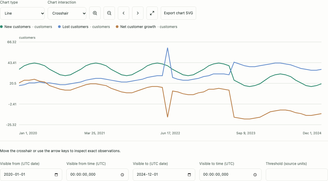
The bundled Illustrative example data covers 60 complete UTC calendar months, January 2020 through December 2024. Customer and MRC balances reconcile. Acquisition and churn have a seasonal cycle, one isolated anomaly in June 2022 and a persistent change from July 2023. Daily customer-base snapshots demonstrate legitimate monthly OHLC. These are synthetic observations, not customer records. The saved measurement, retention rule, signal history and three scenarios use the same engine as your data.
Import your own data
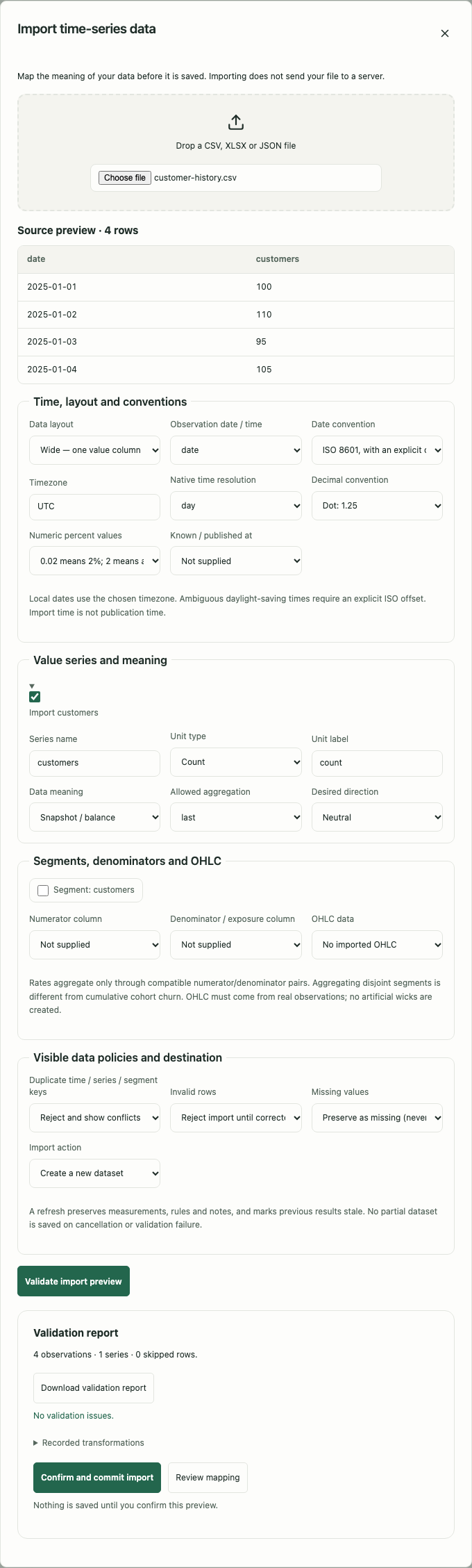
Choose Import your data when creating the template, or open Import in an existing analysis. Choose a local CSV, XLSX or JSON file. Inspect the preview, configure mapping and review the validation report before confirming. Reading a file or generating a preview does not save observations.
Wide and long formats
A wide CSV has a time column and one value column per series:
month,new_customers,lost_customers,opening_customers
2024-01-01,30,20,1000
2024-02-01,32,21,1010
A long CSV has time, series and value columns, with optional segment dimensions:
month,kpi,value,region,numerator,denominator
2024-01-01,churn,0.02,North,2,100
2024-01-01,churn,0.10,South,90,900
JSON accepts an array of row objects with equivalent columns. XLSX maps one explicitly selected sheet. Use the same mappings for equivalent files to obtain the same normalized observations. Formula cells, macros and external workbook links are rejected; imported code is never executed. CSV labels and annotations are text. CSV export protects formula-like text before it reaches a spreadsheet.
Mapping and explicit conventions
Map time, values, series identity and segment dimensions. Where available, also map Known at, numerator, denominator and open/high/low/close. Choose decimal separator, percentage convention, date convention, time zone, resolution, units and each series’ meaning.
- A ratio value
0.02means 2%. In percentage-input mode,2or2%means 2%. - Ambiguous numeric/date values require a convention; they are not silently guessed.
- Date-only values use the selected IANA time zone. UTC ISO timestamps are stored canonically.
- Excel 1900 and 1904 date systems are distinct. The fictional 1900 leap day is not accepted as a real date.
- Ambiguous or nonexistent local times around daylight-saving changes require an explicit unambiguous timestamp.
- Missing observations stay missing. Choose whether invalid rows reject the import or are explicitly skipped; the report identifies rows and columns and records selected transformations.
- Duplicate time/series/segment keys use your selected reject/first/last/keep policy.
Create adds a new dataset. Replace replaces that dataset’s observations. Update replaces matching time/series/segment keys and keeps other observations. Refresh preserves measurement definitions, rules and notes, advances the dataset version and marks affected saved results stale. Retained results keep their original input snapshots; they are not silently recalculated.
Segment selectors list the first 1,000 distinct imported values to keep controls responsive. If a dimension has more values, enter its case-sensitive value in Exact segment and choose Apply exact segment. This also makes values outside the list available without saving each keystroke. Empty values can be selected from the list; clearing an exact-value field removes that dimension filter.
Import and transport limits
The ordinary file limit is 50 MiB; Settings can raise it experimentally up to 1 GiB. Separate analytics limits still apply: at most 200,000 current observations, 100 series, 8 datasets, 200 columns and 10 million input cells. Expanded XLSX content is bounded at 100 MiB. Increasing a file limit does not remove these limits or guarantee that a workbook will fit memory. Parsing/analysis use local workers with progress and cancellation. Cancellation or validation failure leaves no partially saved dataset.
API/MCP has a separate 8 MiB analytics response budget and the bridge’s transport envelope. Prefer paginated data and result queries. A large local file is not automatically an acceptable JSON/base64 request.
Understand time and series meaning
Snapshot/balance means a value at a point in time, such as customer base or MRC. Select first/last explicitly; do not sum balances. Period flow means work occurring during a period, such as new customers; compatible flows can be summed. Rate/ratio needs a definition and, when aggregating, compatible numerator/denominator data. Units, currency, desired direction and definition belong to the series, not its chart.
Disjoint segments with 2 losses out of 100 and 90 out of 900 produce (2+90)/(100+900) = 9.2%.
An unweighted average of 2% and 10% would misrepresent their populations. Combining successive monthly churn
rates does not establish cumulative churn for an original customer cohort; that requires cohort data.
Unsupported temporal rate aggregation is rejected. Net growth and NRR are not artificially capped at 100%.
Customer churn against opening customers uses ratio units, rate semantics and a valid positive risk population.
If a reported rate differs from its supplied numerator/denominator, import preview warns you before confirmation.
The reported value is preserved, including rounding; explicit same-period pooling uses exact exposures.
Observation time, period end and Known at are different. Import time is not publication time. Where historical publication/revision versions are unavailable, validation is explicitly retrospective on the data available now; it does not prove what was knowable in the past.
Chart ranges, measurement intervals, manual trend anchors and Signal Lab cutoffs have separate UTC date and UTC time fields, including seconds and milliseconds. Changing the date preserves the existing clock time; changing the time preserves the date. These fields edit a precise instant, while period aggregation still follows the series’ configured calendar and time zone. Crosshair readouts, observation/publication tables, signal evidence and indicator/residual rows show canonical UTC timestamps so two observations on the same day remain distinguishable.
Explore charts
Choose line, area, bar, candlestick or waterfall. Use time fields, zoom/pan, crosshair and range selection. Keyboard arrows inspect values; chart controls and numeric fields provide alternatives to dragging. Series of incompatible units use separate panels. Normalization is an explicit display choice and never rewrites source observations. Currencies are not added or converted automatically.
Axis ticks use compact display labels; the crosshair and Exact observation details retain the original values and timestamps. If another series has no observation at the inspected time, its nearest sample is labeled with that sample’s actual timestamp. Values outside that series’ observed history are unavailable; the crosshair does not extrapolate or invent an observation.
Candlestick/OHLC requires either validated imported OHLC or at least two distinct actual observations inside
each selected period. Observations 100,110,95,105 produce open 100, high 110, low 95 and close 105.
One monthly churn value cannot produce a meaningful candle or invented wick. If detail is insufficient, the
interface explains the limitation and offers a line chart. Imported OHLC must satisfy low ≤ min(open,close),
high ≥ max(open,close) and finite values. Candles use their original units; choose a line chart for an
indexed/normalized comparison. The interface does not label unconverted OHLC values as an index.
Waterfall uses explicit opening balance, signed change components and closing balance. It verifies the reconciliation rather than treating unrelated series as balance movements. Choose a period to inspect its accounting.
Lower churn can be an improvement even though the number decreases. Read the series’ desired direction, explanation and symbols; color alone is not the interpretation. Historical observations, indicators, measurements, signals and assumption-based scenario layers remain distinguishable. Quantitative analysis is a 2D view.
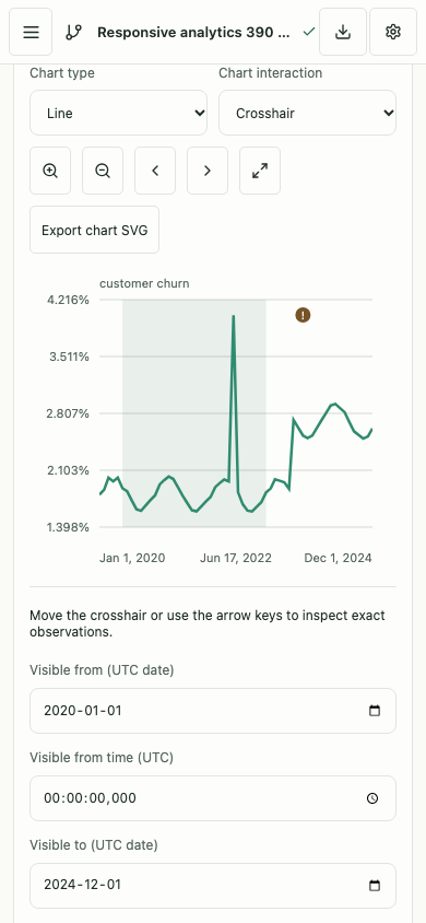
On a phone, the workflow tabs and controls wrap into a compact layout. Open Projects from the app header to switch documents. Use the chart’s interaction selector for crosshair, range selection or pan; numeric date/value fields remain available when dragging would be awkward. Scroll below the chart for additional UTC-time and threshold fields. The expandable observation table provides a text alternative.
Measure change
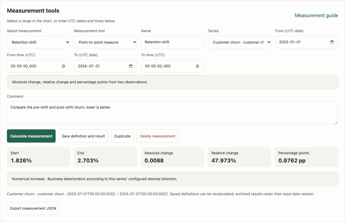
Open Measure. Name a measurement, choose series and time anchors, calculate it and save its definition/result. Selection, numeric fields and exact time/value anchors survive zoom, resizing and chart sampling.
| Tool | What it calculates |
|---|---|
| Crosshair | Exact timestamp, series, value, unit and quality of the inspected observation. |
| Point-to-point | Absolute change, relative change and percentage-point change for ratios. |
| Time range | Elapsed days, calendar periods and actual observation count, separately. |
| Range statistics | Minimum, maximum, mean, median, sample standard deviation, coverage and semantically permitted sum. |
| Trend line | Your two data-anchored points and slope per day; the screen angle is not a slope. |
| Regression | Least-squares fit against actual elapsed time: slope/day, intercept, R², residuals and n. |
| Compare periods | Two explicit intervals; compare totals and means with their lengths, coverage and seasonality in mind. |
| Compare series | Original units or explicitly normalized comparison; incompatible units are not silently combined. |
| Correlation | Pearson or Spearman, matched observations, tie ranks, lag and n. |
| Annotation | A named comment/event tied to its time interval, optionally linked to a diagram node. |
100 → 120 gives +20 and +20%. 2% → 3% gives +1 percentage point and +50% relative change.
Relative change with a zero or negative baseline is reported as not applicable, with a reason; no Infinity is returned.
Normalized series comparison keeps each mean in its original unit: customers remain customers and currency
remains the stated currency. Relative-change results are percentages, not counts or money. Reopened retained
measurements and matching indicator results use their immutable input units even if the current source definition
has changed; they are labeled historical when stale. Changed indicator parameters require recalculation.
Standard deviation uses the sample convention (n−1); insufficient or constant data produces a structured explanation
where a statistic is undefined. Regression uses actual time gaps, not row numbers.
Positive correlation lag means comparing x[t] with a later y[t+lag]; a negative lag reverses that ordering.
Spearman uses average ranks for ties. Missing pairs are excluded explicitly. Correlation does not establish causation,
and no automatic significance claim is made for dependent time-series observations.
A measurement definition is editable and can be recalculated. An archived result is immutable and retains the data/version/parameters used in its calculation. Duplicate, rename, delete or export definitions/results as appropriate; refreshing a source marks old results stale rather than replacing their history.
In Import → Archived runs and retention, edit the maximum saved runs or distinct data-version sets and choose Review retention changes. The review lists the exact runs and attached input snapshots that would be removed. Cancel leaves persisted content unchanged. Confirming the change keeps the newest allowed runs and clears measurement links to removed results while preserving measurement definitions. Deleting an individual saved run uses the same review. Export a document or backup before removal if those historical inputs are still needed; removing local results does not revoke already exported copies or backups.
Detect signals
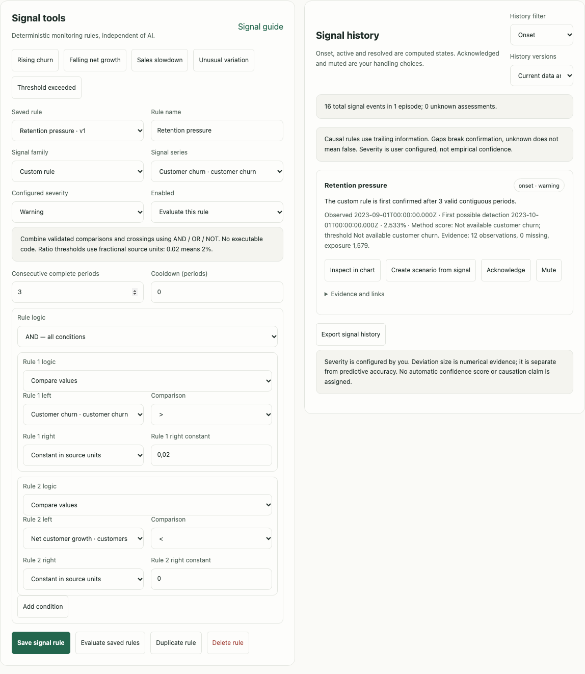
Open Detect, select a business preset or choose a signal family and inspect its parameters. Presets include Rising churn, Falling net growth, Sales slowdown, Unusual variation and Threshold exceeded. Adapt the direction, threshold and exposure to your own KPI definition.
| Family | Definition and main requirements |
|---|---|
| Threshold | Explicit >, ≥, < or ≤ threshold, or crossing up/down and return. |
| Sustained | A condition over N consecutive valid, complete periods; a gap breaks the sequence. |
| Moving-average crossover | A short SMA/EMA crosses a longer one after both are available. |
| Momentum | Trailing relative change against an explicit rolling window and positive base. |
| Anomaly | Rolling z-score or median/MAD against prior observations, excluding the tested point. |
| Variation spike | Observed rolling variation compared with its prior baseline. |
| Structural change | Two-sided CUSUM with explicit baseline μ₀, allowance k, threshold h and reset policy. |
| Seasonality deviation | Current value compared with corresponding seasonal history; at least two complete cycles. |
| KPI divergence | Two specified KPIs move differently under defined change measures. |
| Custom rule | Bounded declarative JSON conditions; no JavaScript, eval or arbitrary formulas. |
SMA/EMA, rate of change, rolling standard deviation, Bollinger-style bands, MACD and RSI are available as exploratory indicators. Their windows and warm-up are explicit. They do not imply buy/sell signals or reliable business thresholds. Short samples and small populations remain limitations, even when changes look large. Without relevant cohort data, the tool does not invent cohort deterioration or leading indicators.
Drag a threshold in Explore, or enter its numeric value, then choose Create signal rule. This opens the same rule definition used by the builder/API. AND/OR/NOT, comparisons, crossing, windows, N-period confirmation, cooldown and hysteresis are declarative conditions. Missing inputs are unknown rather than silently false or zero. For example, churn > 2% for three complete months AND negative net growth can emit Retention pressure.
Signals record their rule/version, data version, interval, observed value, method, evidence, severity and first possible detection time. Onset, active and resolved describe an episode. Rerunning the same rule/data does not duplicate that episode. Acknowledging or muting is your workflow choice and does not change the calculation. Select a signal to focus its interval and inspect why it fired. Severity is configured by you; it is not confidence or empirically measured accuracy. A detected change is not automatically a prediction.
Known at also applies to dependencies. A rule waits for the required secondary KPI or indicator history, then evaluates at its first deciding release. AND-false and OR-true can decide without waiting for an unrelated unknown branch. Delayed earlier periods can complete a current N-period confirmation. Episodes follow the latest published primary observation: late older evidence can complete its trailing window, but cannot resolve or replace a condition already based on newer observations. The observation date is not backdated detection.
History defaults to the current data and rule versions. Choose Earlier data or rule versions or All retained versions to inspect older evidence after a refresh or rule edit. UI and API retain the same bounded history of 10,000 events: linked or handled originals take priority, followed by the newest current and historical events. Any eviction or omitted live event is reported; saved run archives retain their own bounded batch and original inputs. Clear obsolete links/handling explicitly if protected history fills the limit.
Validate in Signal Lab
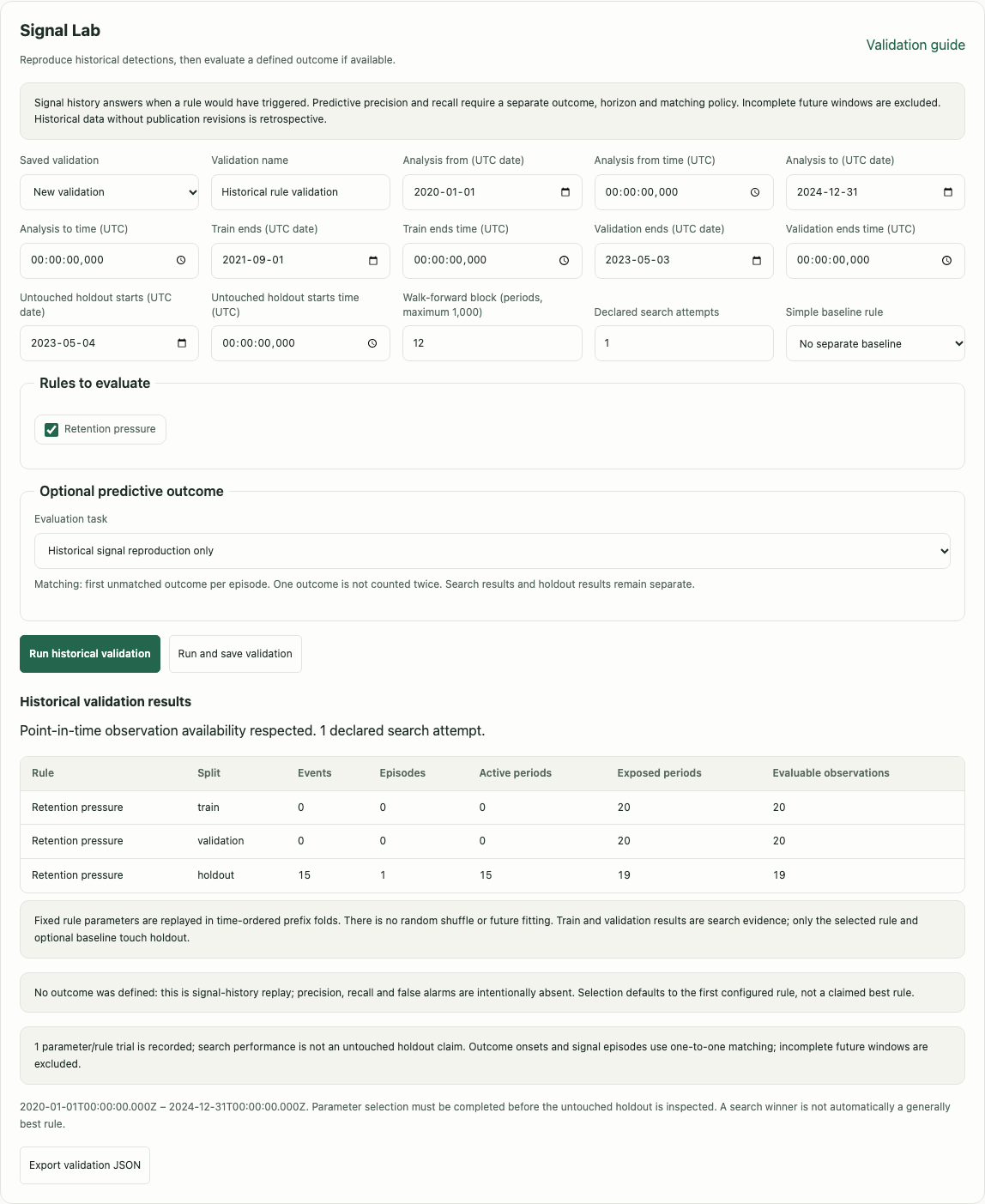
Open Validate to replay rules over history. Choose chronological train, validation and holdout boundaries, a walk-forward size and the number of trials you performed. Each fold evaluates a historical prefix; there is no random shuffle or whole-history fitting of an earlier baseline. A validation-selected rule and optional simple baseline are evaluated on holdout separately. Search performance is not marketed as untouched accuracy.
Each split also replays its final boundary, so delayed dependent data can produce a signal without a new primary observation. For history replay, exposed/evaluable period counts refer to primary observations released during that split. With a predictive outcome, Evaluable instead counts onset signals with complete future outcome windows: the denominator used for precision.
Without an outcome definition, results show signal events, episodes, active periods, exposed/evaluable periods and detection delay. Precision, recall and false alarms are intentionally absent. To assess prediction, define an outcome series, condition, future horizon and first-unmatched matching policy. Complete valid future windows are required; signals/outcomes are matched one-to-one. An outcome occurring before a signal could be known is not a predicted hit.
Outcome episodes use complete published periods in knowledge-time order. Missing, incomplete, unpublished or noncontiguous preceding evidence breaks continuity; the next known qualifying period can begin a new episode. A late release of older evidence cannot create or resolve a stale episode after a newer endpoint is already known. Outcome series must select one explicit segment rather than mixing several populations in the same time key.
Revised data without retained historical publication versions is labeled retrospective. A later analysis may explain an earlier change; it cannot pretend the signal was known then. Saved runs retain their actual input snapshot and configuration. Removing a run/retained version removes that reproducibility evidence; export a backup first if needed.
Compare what-if scenarios
Open Simulate. Compare Baseline, Current trend and Stress scenario over the same future horizon. Edit explicit assumptions, review them and calculate. Scenarios never overwrite historical observations. Fractional customer results are expected counts, not silently rounded individual people.
opening_customers[t] = closing_customers[t−1]
lost_customers[t] = opening_customers[t] × churn_rate[t]
closing_customers[t] = opening_customers[t] + new_customers[t]
                       + reactivated_customers[t] − lost_customers[t]

closing_mrc = opening_mrc + new_mrc + expansion_mrc
              − contraction_mrc − churned_mrc
Churn applies to the opening customer population. New/returning customers are additions after that risk population is defined. MRC is a recurring-revenue balance, not cash flow or recognized revenue. Customer churn only determines churned MRC if you explicitly supply revenue per lost customer; otherwise MRC outflows have their own assumptions.
At 2% churn, +20% relative adjustment gives 2.4%. +0.2 percentage points gives 2.2%. Invalid rates, incompatible currencies and negative populations/balances are rejected with an explanation. Scenario spread is not a statistical confidence/prediction interval.
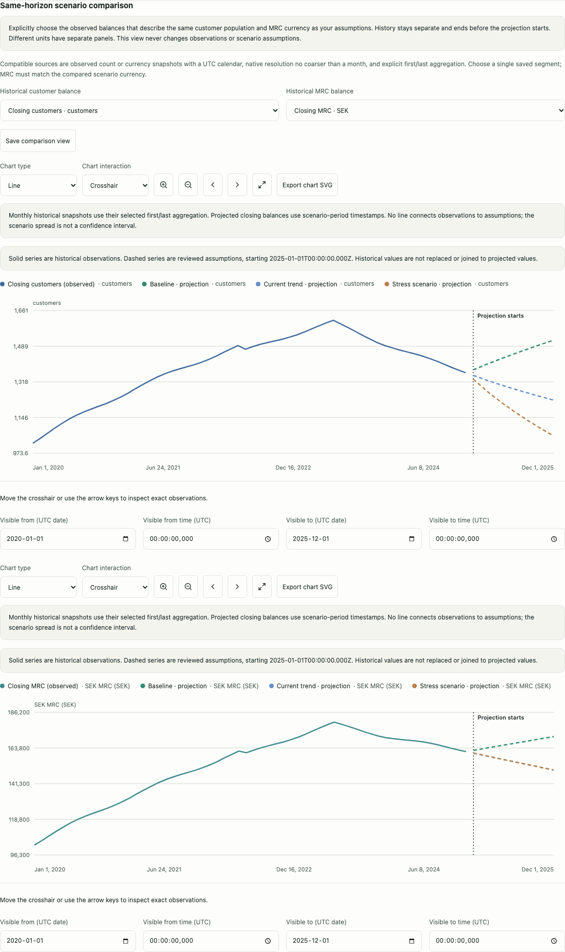
Choose Historical customer balance and Historical MRC balance to place actual observed balances before the projections. Only compatible observed snapshot series are available; MRC must use the scenario currency. This comparison uses UTC months and a selected first/last aggregation from observation-, daily-, weekly- or monthly-resolution history. Other calendars or coarser snapshots are not silently converted or interpolated. These are explicit display sources, not inferred historical values. Use Save comparison view to keep the source choices in the encrypted document. A solid line shows observations, dashed lines show scenarios, and Projection starts marks the boundary. Customer counts and MRC use separate panels and original units. Missing history is left absent, and a different scenario opening balance is not silently substituted for the last observation.
Create scenario from signal opens editable proposed assumptions and the signal evidence. Review them before saving/calculating. The original signal, history and process document are unchanged. Generic node links refer to existing nodes in the current document; the empty example template has no such nodes. The Process Simulator selector can link to another local process document. A process parameter link records its source, target, unit, resolution and review; it does not automatically modify another document or bypass Process Simulator’s existing capacity/queue model.
Save, export and share deliberately
Analytics uses the existing AES-256-GCM encrypted IndexedDB workspace. Raw/derived data, rules, measurements and results have the same vault boundary. Locking clears loaded analysis state and stops workers/jobs. The feature works offline after the normal initial app caching; it does not call AI or send imported business data for analysis.
Use Export chart SVG in Explore for a vector of the currently visible chart, including its displayed layers and rendering sample. This preserves the chart’s current time range and theme. For the complete numerical population, export the dataset as CSV or JSON; a chart drawing is not a substitute for the raw observations. The API/MCP export operation uses the same vector serializer for chart, indicator and scenario views. Exports are bounded to 10,000 displayed points, ten unit panels and 100 saved markers/measurements per panel. Read returned warnings when content is sampled or an overlay is omitted; export numerical data separately for full analysis.
Native document JSON and full backups include the extension and retained result inputs. Plain JSON/CSV exports are readable files; keep them protected. The result retention setting is bounded to 12 archives and three distinct retained data-version sets. Each archive includes its actual input snapshot, so repeated large runs can consume substantial local storage. The complete serialized analytics extension is bounded to 64 MiB. Old runs are removed together with their retained input. Export before reducing retention if you need that evidence.
Live rooms currently reject analytics documents with a clear compatibility message, preserving the extension instead of sending an incomplete model to an older client. Share a deliberate native export or encrypted backup instead. Authorized API/MCP responses and exports can disclose content; local-first is not a promise that data never leaves your browser. Existing backups keep their original password/key and cannot be recalled by changing the live password.
Use REST or MCP
Start the local bridge with the app’s exact origin, for example --allowed-origin https://app.visualnerve.com.
localhost and 127.0.0.1 are distinct browser origins. Your unlocked browser must be available and have a current
Read only or Read + write grant. API/MCP cannot unlock it or renew the idle timer. There are no server alerts
when the app/browser is closed.
For MCP begin with visual_nerve_api_docs and {"document":"guide"}, then request openapi or endpoint for exact
schemas. Use the existing visual_nerve_request, omitting /api/v1 from its path:
{ "path": "/analytics/capabilities", "method": "GET" }
Create the template with write access:
{
  "path": "/diagrams",
  "method": "POST",
  "data": {
    "name": "Growth & Churn",
    "template": "time-series-analysis",
    "mode": "example"
  }
}
Read /diagrams/DIAGRAM_UUID/analytics for compact semantic configuration/current baseVersion, then query raw data
in pages. Dataset/definition changes and saved archives need write access. Pure measurement, indicator, signal,
validation and scenario previews are read-only operations even though they use POST. Long jobs have an ID, progress,
cancel route and bounded results. Saving a job’s result archive is a separate write.
Read the complete executable REST/MCP workflow
and
endpoint schemas
. Capabilities list methods, defaults, warm-up, units and limits. Old bridges lacking
analytics-v1 need a local binary update and client reconnection; a website update does not update that binary.
Version conflicts require reading the current document and reconciling changes. After a timeout, the result may be
unknown: inspect the same operationId and saved state before retrying. Existing operation recovery is bounded to its
original browser/grant and does not promise exactly-once behavior across reloads. Lock or grant revocation cancels
jobs and prevents late results/commits, including after a new unlock. See API/MCP permissions and recovery
.
Methods and limits
The engine is deterministic for the same data, cutoff, definitions, parameters and engine version. Display rounding does not change calculation precision. Undefined statistics return a reason rather than NaN/Infinity. Analysis uses full relevant observations; chart sampling only changes rendering. Two local jobs can run concurrently; result queries are paginated to at most 1,000 rows. Signal Lab has a bounded prefix-replay workload and rejects oversized analyses rather than freezing the browser.
The numerical implementation is documented in the repository’s analytics specification. Relevant methodological references include NIST’s CUSUM definitions , NIST’s EWMA recurrence and time-series cross-validation in Forecasting: Principles and Practice . Our chosen initialization/reset policies are explicit product choices, not a claim of statistical reliability for every dataset.
If a chart or calculation is unavailable, inspect its data-quality message first: missing observations, insufficient history, incompatible units or invalid OHLC are reasons to correct the model, not to invent a value.