Use these Process Simulator examples to ask where a system runs out of capacity, what work waits, and whether a proposed change helps. Every example uses the same saved model and engine as the ordinary simulator. Their numbers are synthetic starting assumptions, not measurements of your equipment.
Choose a starting model
| Template | Useful question | Change first |
|---|---|---|
| API & Compute Capacity | Do requests wait for CPU, retained RAM or a database connection? | Arrival rate, core-seconds/request, pool cores, MiB/request and database slots |
| Network & Multi-Site Capacity | Do uploads from different sites compete for the same link? | Payload bytes, shared Mbps and fixed propagation seconds |
| Energy & Power Capacity | Can generation, the battery and grid supply the requested energy in time? | kWh/job, requested kW, generation windows, battery and grid limits |
| Datacenter Capacity | Does moving one bottleneck expose another across network, compute and energy? | One assumption at a time, then compare the whole completed flow |
- Choose the template under New diagram, name it and create the diagram.
- Open Assumptions. Review the workload, Work steps, resources, connections and scenarios before running.
- Select Base model, then choose Play or Run simulation. MAX calculates the same result without waiting for animation.
- Inspect resource summaries and completion, queue/wait and cost metrics together.
- Save a scenario with one change, run it with the same seed and duration, then compare it with Baseline.
Moving a card changes the diagram layout, not its demand or capacity. See general simulator controls for pause, hierarchy, replay and comparison.
When the controls leave too little room for the process, choose Collapse in the desktop simulator header. Playback, simulated time and status remain visible; Expand restores settings and results without changing the run. On a phone, use Simulation details and return to the canvas when finished. See the compact-panel guide .
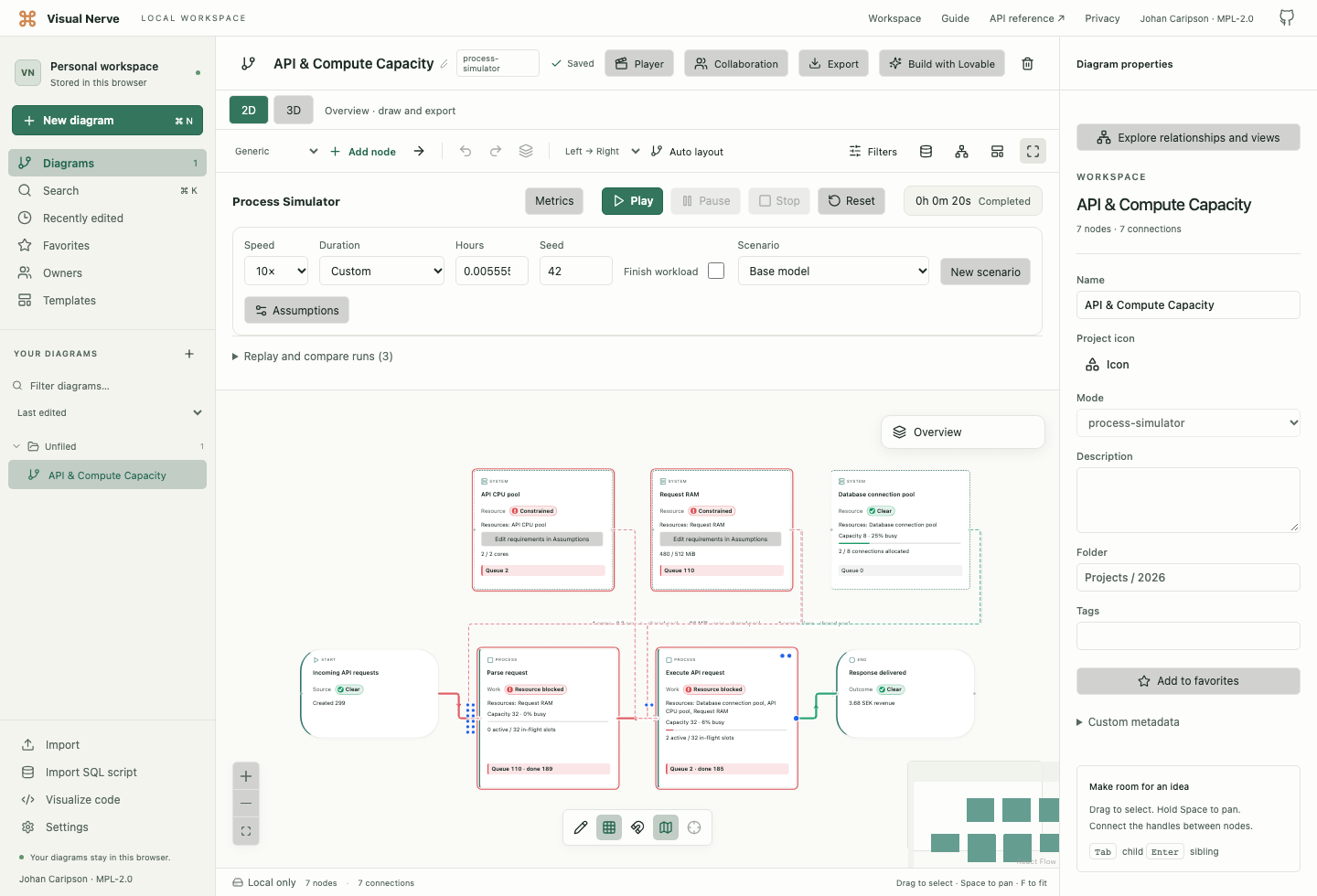
Build through guided setup
- Create an empty Process Simulator. Its Set up your process dialog opens automatically; Start guided setup reopens it when the diagram remains empty.
- In Capacity model domain, choose API & Compute Capacity, Network & Multi-Site Capacity or Energy & Power Capacity. The combined Datacenter Capacity example is available directly from the template gallery.
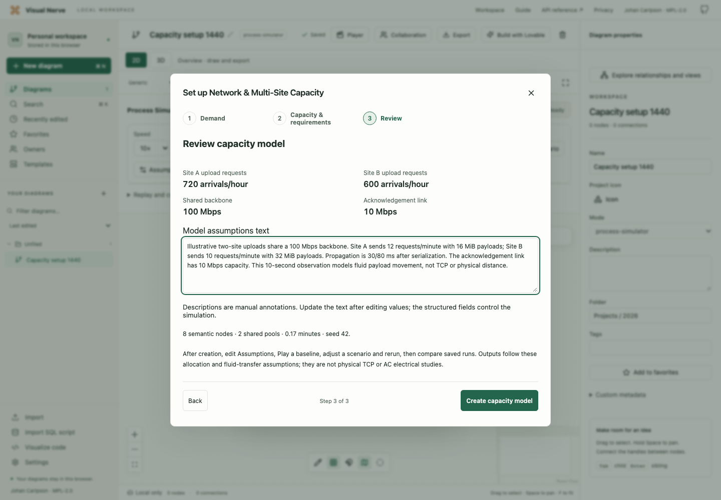
- In Demand, set Run duration, name each source, choose its arrival unit and rate, and set completed revenue. A count of users needs an explicit requests-per-user assumption; it is not itself an arrival rate.
- Continue to Capacity & requirements. Set shared pool capacities, Work parallel slots, CPU/energy activities, RAM leases and network payload/propagation fields. The pools remain shared across every referring step.
- Use each quantity’s unit selector deliberately. MiB/GiB are binary memory sizes, Mbps/Gbps are decimal link rates, and kW and kWh measure power and energy separately. Invalid numeric drafts show an error and prevent continuation.
- Continue to Review. Check the current source arrival rates, pool capacities, node/pool counts, duration and seed. Model assumptions text is a manual annotation: update it to describe your edited values, then use Back if a structured field needs changing. Create capacity model applies one undoable graph/model change. Closing the dialog leaves the existing diagram unchanged.
Edit the saved assumptions
Select Base model and open Assumptions, or select a saved scenario before opening it to edit that scenario’s resolved assumptions. The same editors save the model used by UI, REST and MCP.
| Editor section | What to change |
|---|---|
| Nodes | Choose a Source to edit arrivals. Choose Work for Work capacity, Activity dimension, Computational work, Cores per active request, Fixed processing overhead, Energy per item, Requested load power and RAM leases. |
| Resources | Choose the Resource dimension, pool capacity and cost. Energy pools also expose generation windows, grid import, price/kWh and battery bounds/efficiencies. Keep a database connection pool as a General shared resource. |
| Connections | Enable Network transfer, select its bandwidth pool, then enter Payload and Propagation delay. |
| Processes | Organize scopes without adding processing or copying resource capacity. |
| Improvements / Economics | Enter supported interventions and costs, with one currency per model. Energy demand changes use explicit energy/power fields. |
For a generic database pool, use the Work section Shared resources required together to require one connection alongside its CPU/RAM allocation. Add or remove typed requirements through these domain editors; their dashed dependency lines disclose the requirements and cannot be edited independently as particle-flow connections.
Choose Apply assumptions to validate and save the complete change. Invalid drafts or unsupported combinations do not partially save. A new run captures the new assumptions, while saved older runs keep their original model.
With Base model selected, expand Model assumptions and edit Model assumptions text to describe synthetic inputs, user-to-request conversion, units and limitations. This text is saved with the model, but it does not set rates or capacity; the structured fields do. Update it after changing numbers. Scenarios keep the baseline annotation; give each scenario a name that identifies its changed assumptions.
API requests: dedicated CPU and retained RAM
CPU Work reserves its requested cores, together with newly needed RAM, when the complete allocation is available. It waits otherwise. Work capacity limits simultaneous jobs at that step; CPU pool capacity limits dedicated cores across all its jobs. This is an allocation model, without CPU timeslicing.
Without complexity or improvement multipliers, service time is:
fixed processing seconds + core-seconds / allocated cores
For example, 0.2 core-seconds on one core plus 0.015 seconds of overhead needs 0.215 seconds. Reserving two cores for that request reduces the compute part to 0.1 seconds while retaining the fixed overhead. Increasing only the pool’s capacity permits more concurrent requests; it does not change each request’s reserved cores. Complexity and applicable improvements multiply the modeled duration; these are explicit assumptions.
Stage RAM is released when that Work step ends. Case RAM stays with the original request through later steps, CPU waits and network travel. Repeating a case demand tops it up to the largest requested amount for that request and pool; it does not allocate another copy each time. Forked branches share that retained case allocation. A step can separately need stage RAM too.
Try increasing CPU while leaving RAM unchanged. If requests still wait because retained memory fills the pool, more CPU alone will not remove that limit. Compare reserved cores, peak/used MiB, retained leases and completed requests. Occupied core-time includes fixed overhead; completed CPU work is a separate counter.
The starter also has eight shared database connection slots. Execute API request holds one connection atomically with its CPU allocation and releases it after execution; RAM stays with the request until final completion. The One database connection scenario increases CPU/RAM headroom while reducing database slots to one. It helps distinguish a connection limit from a compute or retained-memory limit. This is a connection-pool assumption rather than a database I/O simulation.
Multi-site links: payload and propagation
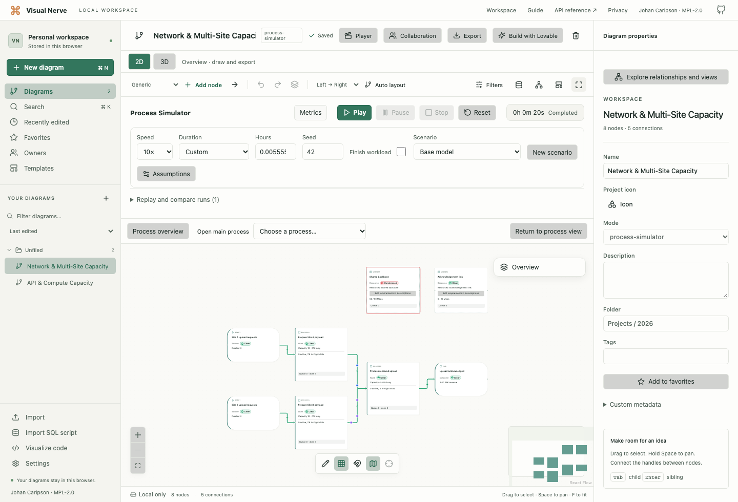
Put every flow using the same physical or assumed bottleneck on the same typed link resource. Concurrent transfers share its available bandwidth equally. Shares change as transfers start or finish, so two sites compete even when they are drawn in separate process groups.
One Mbps is 125,000 bytes/second. With one active 1,000,000-byte transfer on a 10 Mbps link, serialization takes 0.8 seconds. Two equally active transfers each get half the rate until one finishes. The connection’s fixed travel time is added once after serialization; it is separate from payload size.
Try reducing payload size, increasing shared Mbps, or changing propagation independently. Inspect active transfers, transferred bytes, used Mbps, downstream queues and completed cases. Bandwidth schedules can change availability; automatic link scaling is not supported in this version.
An active transfer on a zero-capacity or currently closed link is Constrained, with the explanation Active transfers have no currently available bandwidth. Its zero measured use means that serialization cannot progress, rather than that the link has no demand. The bottleneck is the link; a pending transfer does not create an invented Work queue. The constraint clears when bandwidth becomes available or the transfer ends. Idle links and particles whose payload has finished and is only propagating do not receive this marker.
The model does not infer distance, TCP behavior, packet loss, retransmission or congestion control. Enter measured or deliberately chosen assumptions for payload and latency.
Energy: power determines speed, energy determines completion
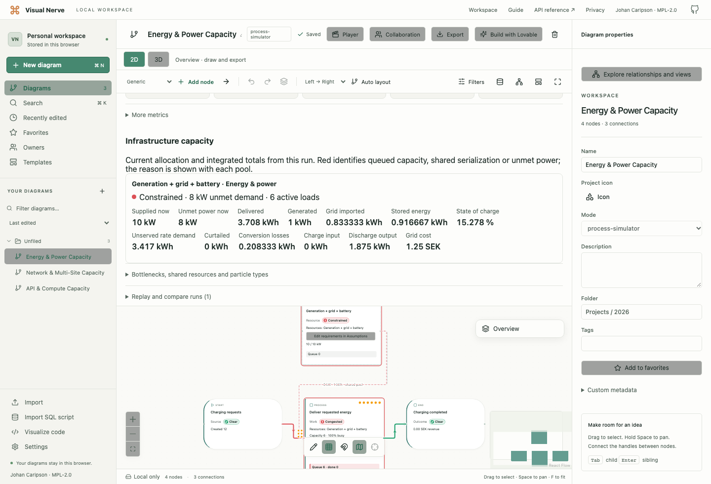
A job requesting 1 kWh at up to 3 kW takes at least 20 minutes when it receives the full 3 kW. Less delivered power extends completion time. A large battery stores more energy, but its discharge-power limit can still restrict how quickly it supplies loads.
The energy pool’s capacity is the maximum power delivered to loads. Generation windows, battery discharge limits and maximum grid import describe the available supply separately. Gaps between generation windows produce zero generation.
The engine uses generation first, battery discharge second and bounded grid import last. Loads share available power fairly: small requests receive up to their requested power, then the remaining supply is shared equally among larger requests. Generation surplus charges the battery within its energy/power limits and efficiency; remaining surplus is curtailed. Grid imports do not charge the battery in this version.
Compare delivered/imported kWh, stored energy, state of charge, conversion losses, curtailed energy and unmet requested power. Unserved kWh measures requested power that could not be delivered at that rate over time; a slowed job may still receive the remaining energy later. Grid cost uses imported kWh and the configured price/kWh, in the model’s currency.
Try a larger battery, a higher discharge limit, more grid import or a different generation window as separate scenarios. Energy Work uses delivered energy instead of a fixed processing time. Energy supply is controlled by explicit windows; resource schedules and automatic scaling are unsupported.
This is an aggregate energy balance. It does not calculate AC voltage, frequency, protection, battery chemistry or weather-derived solar/wind production.
Combine the domains carefully
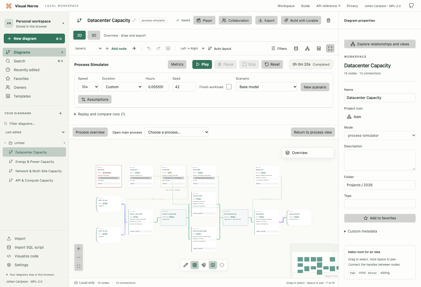
Datacenter Capacity combines WAN transfer, retained RAM, CPU, an energy budget and database connections. After receiving a request, a fork starts CPU computation and its explicit energy budget concurrently. The paired join waits until both branches finish, then the request uses a database connection and sends its response. There is no automatic conversion from CPU usage to electrical energy; that budget is a separate stated assumption.
Follow a request from arrival to final completion. A faster link can shift waiting to compute; insufficient power can hold the join even after CPU computation finishes. Retained case RAM follows the original request through both branches and the response. Compare the whole result instead of adding overlapping process totals or treating a green upstream card as proof of end-to-end capacity.
Read a run honestly
Model 2 Work cards show one logical step with its in-flight capacity, active jobs and queue. Those concurrency slots are not physical server replicas. All resource cards show one aggregate pool, including generic database connections and typed cores, MiB, Mbps or kW. Legacy simulator models retain their earlier capacity-card banks. The metrics come from the actual engine state.
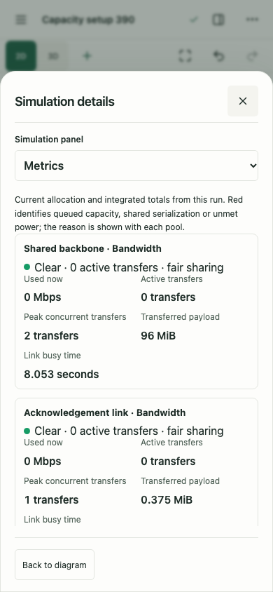
- Use Metrics on desktop, or Simulation details → Metrics on mobile. Scroll to Infrastructure capacity for each typed pool’s named Clear, Busy or Constrained reason and measured quantities.
- Compare current and peak allocation with cumulative totals. A completed finite observation can have active jobs or transfers left; a pool’s zero current use does not erase its earlier peak.
- Read the bottleneck’s reason with its queue and completion data. Resource constraints come from actual blocked admission, concurrent link sharing or unmet power; a request waiting on CPU does not by itself prove that RAM is constrained.
- Select a saved scenario and run it with the same seed and duration as Baseline. In Replay & compare, compare saved runs, then expand Infrastructure comparison and a pool to read Baseline, Scenario and signed Change values.
- A dash means that pool has no corresponding measurement on that side, rather than an invented zero. State of charge changes use percentage points. Inspect global completion, wait and cost metrics alongside the domain table.
A finite-duration run observes that interval and may leave work outstanding. If Finish all generated work cannot make further progress, the run fails with SIMULATION_INFRASTRUCTURE_STALLED and preserves partial totals. Check zero capacity, an unsatisfiable atomic demand, exhausted supply and missing future availability. Failure releases allocations; it is not successful completion.
Case memory can be explicitly released after a stage outside fork/join regions, or automatically at final completion, failure or cancellation. Releasing it inside a parallel region is rejected because other branches may still use it.
API and MCP use the same assumptions
Use bridge/browser 0.10.0 with infrastructure-resources-v1, then read GET /simulation/capabilities. Legacy models remain version 1. Infrastructure models require schemaVersion:2 and infrastructure:{schemaVersion:1} together so older clients reject unsupported execution.
Use the existing simulation model/entity CRUD, asynchronous run, state/result and comparison routes. Read only permits inspection and comparison; changing a model or starting a run requires Read + write. Versioned PATCH preserves omitted fields, recursively merges objects, removes optional fields with null and replaces arrays. Complete/new models reject null and invalid assumptions atomically.
Live collaboration rooms currently reject infrastructure models. Share an explicit native JSON export or encrypted backup instead. The workspace remains local and encrypted; API traffic neither unlocks it nor renews its idle timeout.
See API/MCP setup , the API reference and the simulator guide for endpoint schemas, run controls and privacy rules.