Process Simulator helps you ask a whole-system question: “If demand, staffing or processing changes, what happens to queues, customers and cost?” Build assumptions explicitly, run them, inspect the results and compare a scenario with its baseline.
It is a separate Process Simulator template and document type. Ordinary diagram placement controls presentation; moving a card does not change arrival rates, processing times, resource requirements or routing.
For API/CPU/RAM, shared multi-site links, generation/grid/battery supply and a combined datacenter flow, use the infrastructure capacity guide . Those examples keep these controls and add explicit typed resource assumptions.
Build a process from scratch
- Choose New diagram → Process Simulator → Create diagram. An empty process opens Set up your process.
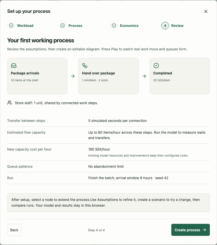
- In Workload, name the work item. Choose a regular arrival rate or a finite batch, then set the simulation length.
- In Process, choose One work step or Main process and subprocesses. Name the steps, set minutes per item and parallel capacity, and choose travel time between steps. Optionally add shared staff or equipment.
- In Economics, set the currency, revenue per completed item and hourly operating costs. Set a maximum queue wait if waiting work may abandon.
- Review the assumptions and choose Create process.
- Choose Play. The initial 10× speed makes movement visible; use 1× for closer inspection or MAX to calculate results quickly.
The single-step wizard creates a connected Arrivals → Work → Completed model. The subprocess option creates a main process containing an ordered flow of individually configured steps. A shared resource appears as a separate capacity card with dashed requirement links. All assumptions are saved in the same simulation model used by the API and MCP.
Choose Set up later to leave the canvas empty. Start guided setup reopens the wizard. Applying setup creates the model in one undoable operation; closing the wizard leaves the existing document unchanged.
Extend directly from a node
Select a node and use Add next beside it. A new step and its connection are created together. If a Source or Work step already has one outgoing connection, adding a Work or Decision step inserts it into that path. A Decision can add an alternative branch. Add previous extends an Outcome; Add work on a Resource creates a Work step using that same shared capacity.
New Work steps start with one slot and one minute of processing. New process connections have three seconds of real transfer time. Open Assumptions to change those values, resource requirements or routing rules. Undo removes the added node and connection together.
Main processes and subprocesses
Use process groups to keep a large model understandable without hiding where work really waits. A group can contain more groups and actual Source, Work, Decision or Outcome steps. Work steps retain their own times, capacities, costs, queues, routing and shared-resource requirements. A group adds no extra processing or charge.
Create a hierarchy with guided setup
- Start an empty Process Simulator and complete Workload.
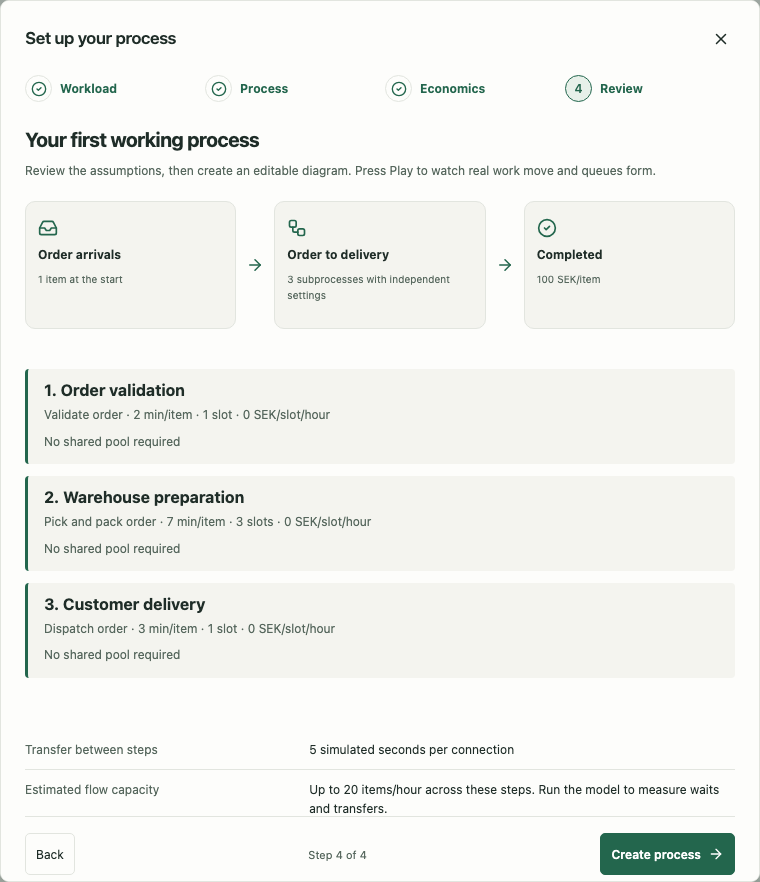
- In Process, choose Main process and subprocesses and name the main process.
- Configure each subprocess’s name, Work step, minutes per item, parallel capacity and hourly slot cost. Add subprocess adds another ordered stage; Remove removes a draft stage.
- Enable the shared pool if needed. Choose Use shared resource in this step only for the stages that require that pool. These stages compete for one pool, rather than receiving separate copies of its capacity.
- Review each stage and its resource assignment. Choose Create process.
- Choose Open process on the main card, then open a subprocess to edit its real Work step. Add step creates work in the open group; Add next beside a selected step keeps its process membership.
The wizard supports one to twelve sequential subprocesses. After setup, use Assumptions → Processes to add deeper levels or parallel groups, then configure connections and routing for the actual steps.
Open, edit and navigate a process
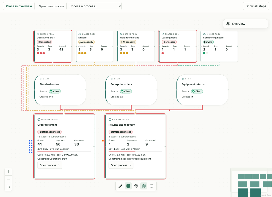
Process overview shows the main groups and the shared pools. Choose Open process or double-click a group. The navigation’s Open main process and Open subprocess selectors reach a group directly, including on a phone. The breadcrumb shows your current location; choose a parent name to move up. Show all steps displays the complete underlying flow, and Return to process view restores the hierarchy.
Under Assumptions → Processes, add a main process or subprocess, edit its name and description, choose a parent, or assign existing steps. The Process group field in a node’s settings changes its membership. Removing a group keeps its real work and moves members to its parent or the overview. Invalid references and cyclic nesting are rejected.
Hierarchy views arrange the visible cards compactly. Shared pools show actual capacity, busy units and queued work in a single summary card. On a phone, opening a group focuses a readable child card; pan to inspect its neighbours or use Fit diagram for the full view. Use Show all steps to edit the full flow’s placement. 3D, presentations and exports show the complete real flow. Return to 2D for the collapsible hierarchy. Groups and capacity displays are temporary visual projections; they do not become additional simulated work.
Read congestion at both levels
A group card shows its actual current queue, work in the process, completed visits, average wait, cycle time, allocated cost and named constraint. Green, yellow and red reflect observed state. Open a red group to find the constrained Work step or shared pool. Items crossing a group boundary follow their real connections; internal movement becomes visible when the group is open.
Parent values include their descendants. Do not add a parent and child total together. Completed on a group means a successful visit that left that group or finished at an Outcome inside it; the system’s Completed count means final successful Outcomes. Group cycle time measures entry to exit, and group TTR measures entry to a revenue Outcome. System TTR measures creation to revenue.
Group costs include its Work operations and the occupied units of shared resources consumed there. Idle pool costs, shared scaling overhead and investment remain in system totals. Revenue appears in the Outcome’s group and its ancestors. These rules avoid charging the same item repeatedly as it passes through stages; whole-system economics remain the comparison reference.
Explore delivery operations and returns
- Choose New diagram → Delivery network + returns → Create diagram.
- Run Baseline at MAX to calculate eight opening hours, or at an animated speed to inspect work movement.
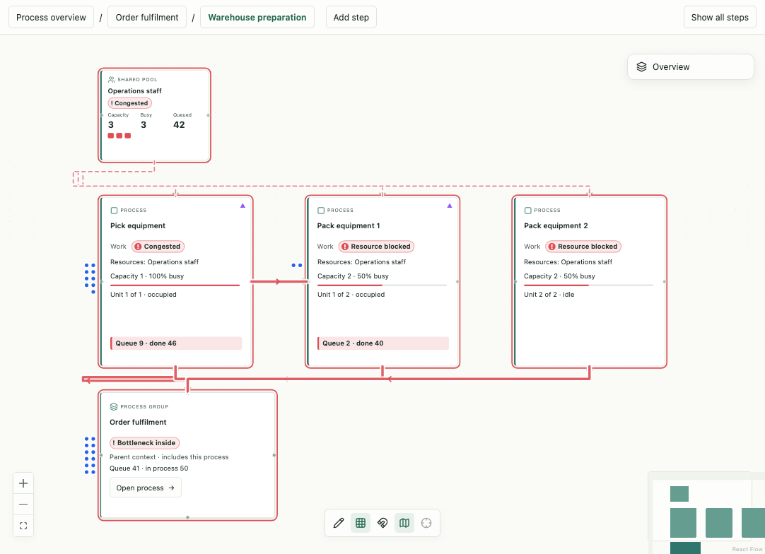
- Open Order fulfilment → Warehouse preparation. Compare picking and packing queues with the shared operations pool.
- Return to the parent and open Delivery and installation → Transport or Field service to inspect downstream constraints.
- Run 10× returns, same staff. Returns share operations staff, the loading dock and technicians with deliveries.
- Run Expand warehouse capacity, then Expand warehouse and field delivery, and compare completed work, wait, cost and contribution. Extra capacity is paid at the configured rates.
The example has 23 real nodes, 11 process groups, three item types and five shared pools. Standard orders arrive at 18/hour, enterprise orders at 4/hour, and returns at 2/hour during an eight-hour opening day. Enterprise work has higher complexity and an additional design step. All times, revenues, patience limits, resource prices and scenarios are editable in Assumptions. These are illustrative assumptions, not business recommendations.
The Assisted picking investment scenario enables a 250,000 SEK improvement that reduces picking time to 65% and adds 20 SEK/hour operating cost. Compare it with the baseline: if the investment does not pay back within the captured period, the result says so.
Build the same hierarchy through API or MCP
Create groups through POST /diagrams/{id}/simulation/processes, set parentId for nesting, and assign real nodes with processId. GET .../simulation/hierarchy returns semantic membership independently of canvas coordinates. GET .../simulation/runs/{runId}/processes/{processId} exposes the same queue, timing, cost and bottleneck values shown on group cards. See API/MCP
and the API reference
for versioned writes, validation and runnable examples.
Run the kiosk example
- Choose New diagram → Kiosk + package pickup → Create diagram.
- Read the example’s assumptions under Assumptions.
- Choose a Scenario, Duration and Seed.
- Choose Play and watch the 2D diagram. Fit diagram shows the whole process in the space available below the dashboard.
- Inspect the metrics, queues and shared resources.
- Run a different scenario with the same duration and seed.
- Select the saved runs and choose Compare selected runs.
The desktop dashboard groups key numbers into cards and identifies the current bottleneck. More metrics expands queue statistics, lost work and further timing measures. Use Metrics beside the playback controls to hide or show the dashboard without changing the run; hiding it gives the process canvas more space. Replay and comparison remain below the metrics.
Give the diagram more room
On desktop and larger tablets, choose Collapse in the simulator header to fold the full control panel. Play/Resume, Pause, Stop, Reset, simulated time and run status remain available in a compact strip. Duration, seed, scenarios, metrics and replay/comparison move out of the way, giving the diagram more space.
Folding is a view change: it does not pause or restart a run, change its assumptions or save a new model. Choose Expand to return to your settings and replay/comparison choices. Errors and notices remain visible while folded. The choice stays with the currently open diagram, including switching between 2D and 3D, and resets when you open a different diagram, reload or lock the workspace.
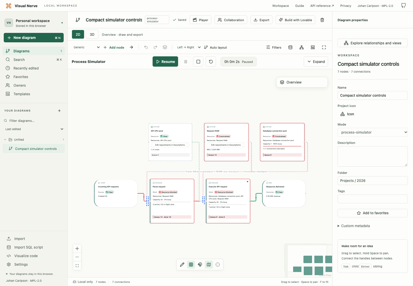
On a phone or short landscape screen, use the existing Simulation details sheet for settings, metrics and saved runs. Closing that sheet returns to the canvas; the compact playback strip remains available.
Read the process like a traffic map
Flow connections show the pressure at the next step: green means clear, yellow means busy or a queue is forming, and red means work is queued behind saturated or blocked capacity. Nodes also show words, symbols, actual queue counts and utilization, so color is not the only signal. A shared resource can make a Work step red even when that step has free slots.
Work items keep their particle type’s color and shape while traveling along valid process connections. Travel uses the model’s transfer time; a zero-second transfer is instant. A small sample waits beside a congested step, while its queue label counts the complete workload. Dashed resource requirements carry no particles.
Use Pause to inspect a traffic jam. It freezes the simulation and particle movement together. The renderer interpolates observed simulation timestamps; it never creates extra throughput. MAX calculates the same business result without waiting for animation.
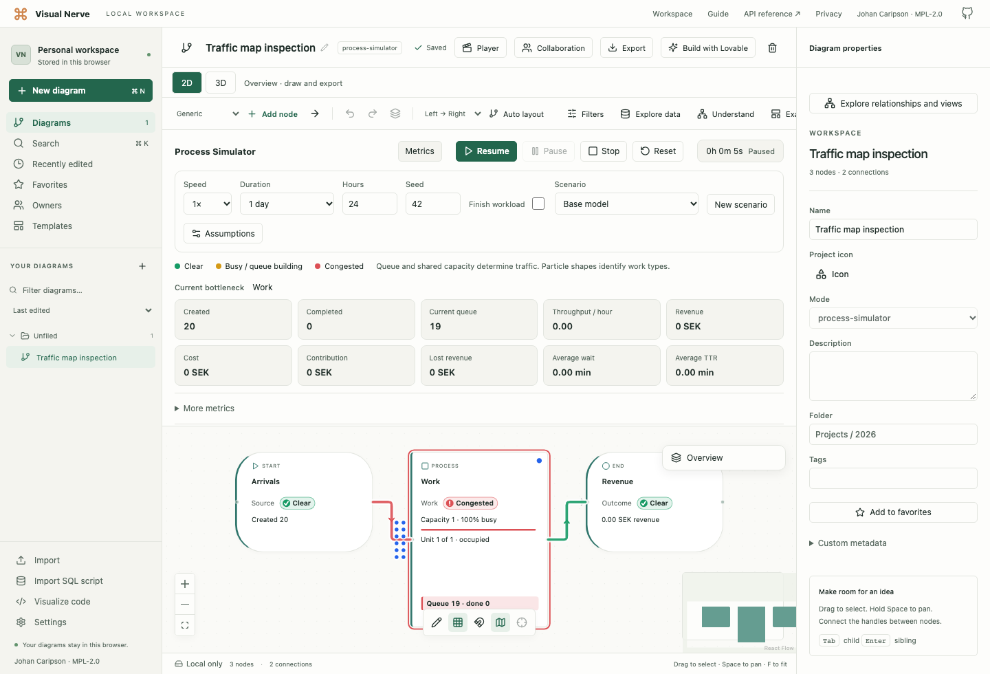
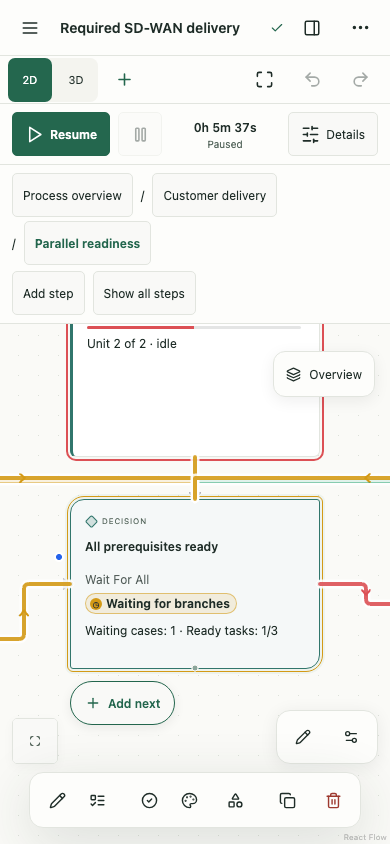
On a phone or short landscape screen, Play, Pause and simulated time stay in a compact canvas strip. Open Simulation details to choose Run settings, Metrics or Replay & compare. Run simulation starts the configured run and returns to the diagram.
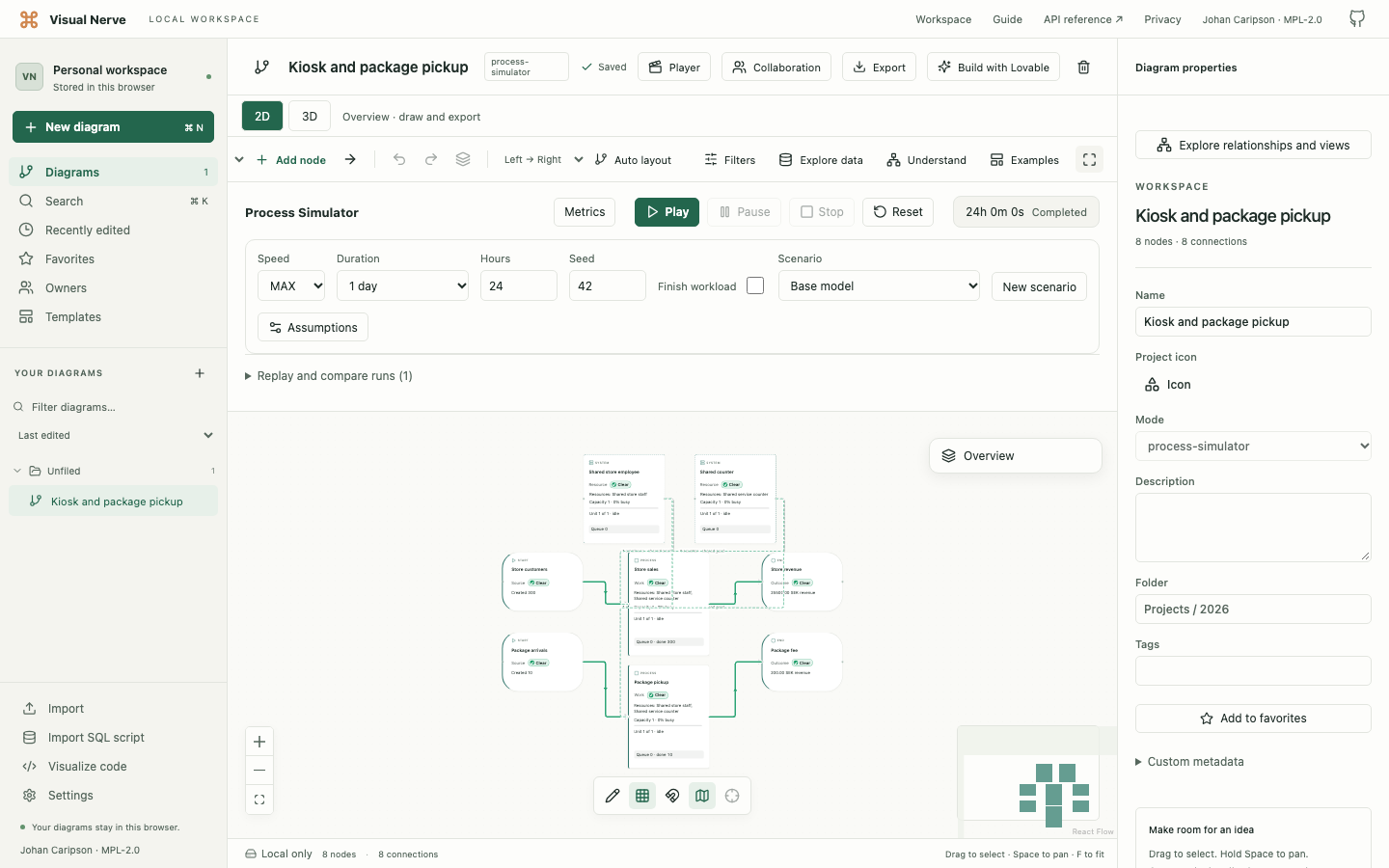
Understand the example before drawing conclusions
The bundled kiosk assumes a repeating 12-hour opening day followed by 12 closed hours:
| Assumption | Store purchases | Package pickups |
|---|---|---|
| Arrivals per opening day | 300 | 10 |
| Processing time | 2 minutes | 4 minutes |
| Revenue per completed item | 85 SEK | 20 SEK |
| Queue patience | 4 minutes | 8 minutes |
| Required shared capacity | One employee and one counter | One employee and one counter |
Arrivals are evenly spaced. Each process connection adds three seconds of travel. Shared staff costs 180 SEK/hour while scheduled available. These are illustrative, editable assumptions.
Store work requires 600 processing minutes and baseline package work requires 40. One eight-hour employee cannot provide 640 minutes. The example makes its 12-hour assumption visible rather than hiding this capacity shortfall.
Bundled scenarios expose different constraints:
- 1,000 packages/day increases package pressure on shared staff and counter.
- +1 package employee assigns packages to paid package staff while retaining shared-counter contention.
- +2 package employees and dedicated counter provides parallel package processing and removes package demand from the shared counter.
Compare package throughput with store waiting and lost revenue, not only package completion. Added paid capacity carries its configured cost, and a bottleneck can move to another part of the system.
Understand the model’s building blocks
| Building block | Meaning |
|---|---|
| Particle type | A kind of work item: customer, package, order or job, with revenue, complexity, priority and patience. |
| Source | Generates that work according to arrivals, a burst, schedules and limits. |
| Work | Processes queued items using its own parallel slots and required shared resources. |
| Parallel work | Starts every required branch for the same case. |
| Wait for all | Resumes that case when all of its paired branch tasks arrive. |
| Router | Chooses a valid outgoing route using rules or current state. |
| Resource | Shared capacity such as staff, counters, machines or vehicles. Multiple Work nodes can compete for it. |
| Outcome | Completes, fails or rejects work, and can realize revenue. |
| Process group | A main process or subprocess containing real steps and nested groups; summarizes observed behavior without adding work. |
| Process connection | A permitted flow path with a travel time. |
| Improvement | An investment or operating change affecting a Work/Outcome node or resource. |
Dashed resource connections represent capacity requirements. They are distinct from particle-flow routes. A resource can be part of the model without a visible canvas shape; add its resource display if you want to place it in the diagram.
Edit assumptions safely
Open Assumptions, which opens Process Simulator settings. Desktop has sections for nodes, processes, connections, particles, resources, improvements, economics, complete model. On a phone, use Settings section to select one.
Changes remain a draft until Apply assumptions. Cancel discards the draft. Invalid JSON or invalid semantic references must be corrected before applying. If the saved model changes while this editor is open, reopen it against the current version.
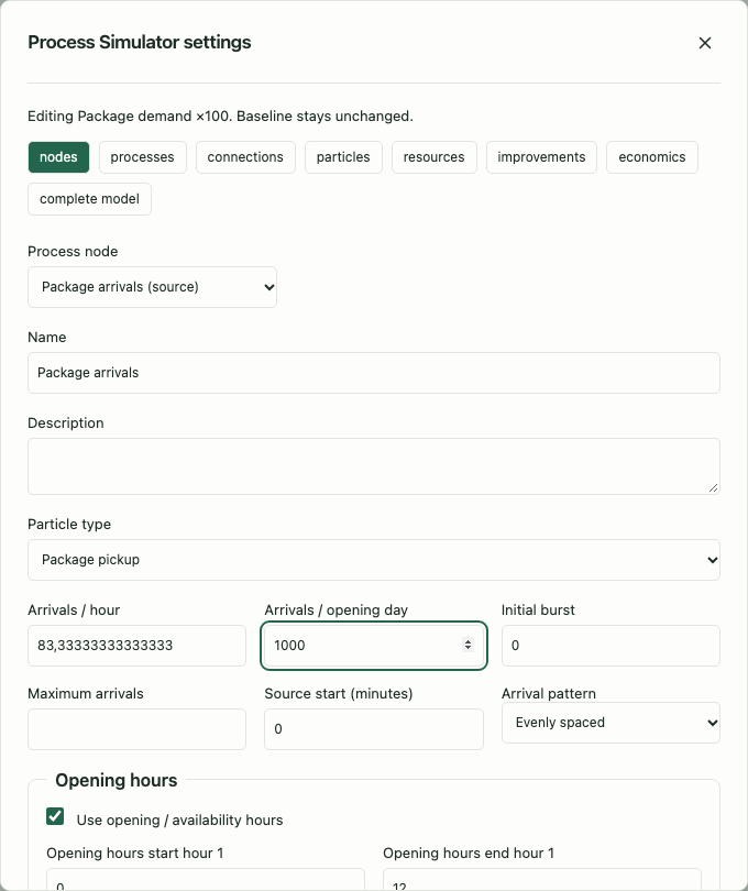
The editor labels units: processing and patience use minutes where shown, availability uses hours, and connection travel uses seconds. The underlying model/API use simulated seconds. Arrival rates and operating costs are per hour; money uses the model’s three-letter currency code.
Particle types: value, complexity and patience
In particles, choose Particle type to edit or Add particle type.
- Name, Color and Shape identify the work in the animation.
- Revenue is its initial expected value.
- Minimum complexity / Maximum complexity determine processing requirements together with Work settings.
- Priority matters when a Work queue uses Particle priority; higher priority goes first, with arrival order breaking ties.
- Patience (minutes) limits how long it can remain waiting in a Work queue. An omitted value does not impose that patience limit.
- Attributes provides structured values that routing rules can test.
Deleting a type in the baseline draft also removes sources that generate it. Apply the reviewed draft as one undoable operation.
Sources: arrivals and opening schedules
In nodes, select a Source and configure:
- Particle type.
- Arrivals / hour or Arrivals / opening day.
- Initial burst, Maximum arrivals and Source start (minutes).
- Arrival pattern: Evenly spaced or Random arrivals (seeded).
- Opening hours and Use opening / availability hours.
Daily/weekly repeats let a multi-day simulation keep generating work. Once describes a single window. Multiple windows can represent separate shifts.
Use Maximum arrivals only when the source should have a finite total. A source intended to produce the same daily volume throughout a week should have a repeating schedule without an accidental one-day maximum.
Arrivals per opening day is calculated from the configured opening-window hours. Verify those hours before interpreting a daily rate.
Work: processing slots, queue and required resources
Select a Work node in nodes.
| Setting | Effect |
|---|---|
| Work capacity | Number of its parallel processing slots. |
| Processing time (minutes) | Base processing duration, modified by complexity and enabled improvements. |
| Complexity multiplier | Adjusts the effect of work complexity. |
| Work cost / hour | Cost per available capacity unit, including idle time. |
| Cost / processed item | A per-item processing charge. |
| Maximum queue | Limits waiting items. |
| Queue order | First in, first out, or Particle priority. |
| Overflow route | Abandon when full, or route to an actual connected destination. |
| Accepted particle types | Limits compatible work; empty means all types. |
| Shared resources required together | Resource units the item must acquire together before processing. |
| Work availability | When the Work capacity is available. |
For example, three processing slots still cannot process three simultaneous items if each requires the same single employee and single counter. All required resource units must be available together.
An overflow or failure route must correspond to a real outgoing flow connection. Draw or configure that connection before choosing it.
Shared resources: capacity, cost and availability
In resources, choose Resource to edit or Add shared resource. Configure its name, unit, capacity, minimum/maximum, hourly cost, scaling and availability.
If store sales and package pickup both require the same employee resource, they compete for its capacity. Adding a second Work card does not invent another employee.
Hourly cost is per available resource unit, including idle available time and active overtime outside availability. A required resource’s closed schedule can prevent processing even when the Work node itself is open.
Deleting a resource in the baseline draft also disconnects its Work requirements and removes related resource displays and investments. Review the draft before applying.
Routers and process connections
In connections, add a process connection with From, To and Connect process nodes, or edit its travel time. Native flow connections remain editable; their permitted endpoints determine valid routing paths.
For a Router, choose a Routing strategy:
| Strategy | What it chooses |
|---|---|
| first-match | The first matching rule in configured order. |
| weighted | An eligible rule using relative positive weights. |
| least-queue | A compatible route using queue state. |
| available-capacity | A compatible route using available capacity. |
Add routing rule chooses a destination and optional condition. Conditions can use particle type, complexity, priority, revenue, an attribute, queue, available capacity or utilization. State conditions specify the Work node or resource to inspect.
Set Fallback connection deliberately. Weighted routing with no positive eligible branch uses a valid type-compatible fallback; if none exists, the particle fails rather than following an invented route.
A Router chooses one continuation. Use Parallel work when the same case needs several tasks to finish before it can continue.
Parallel tasks: wait for the same case
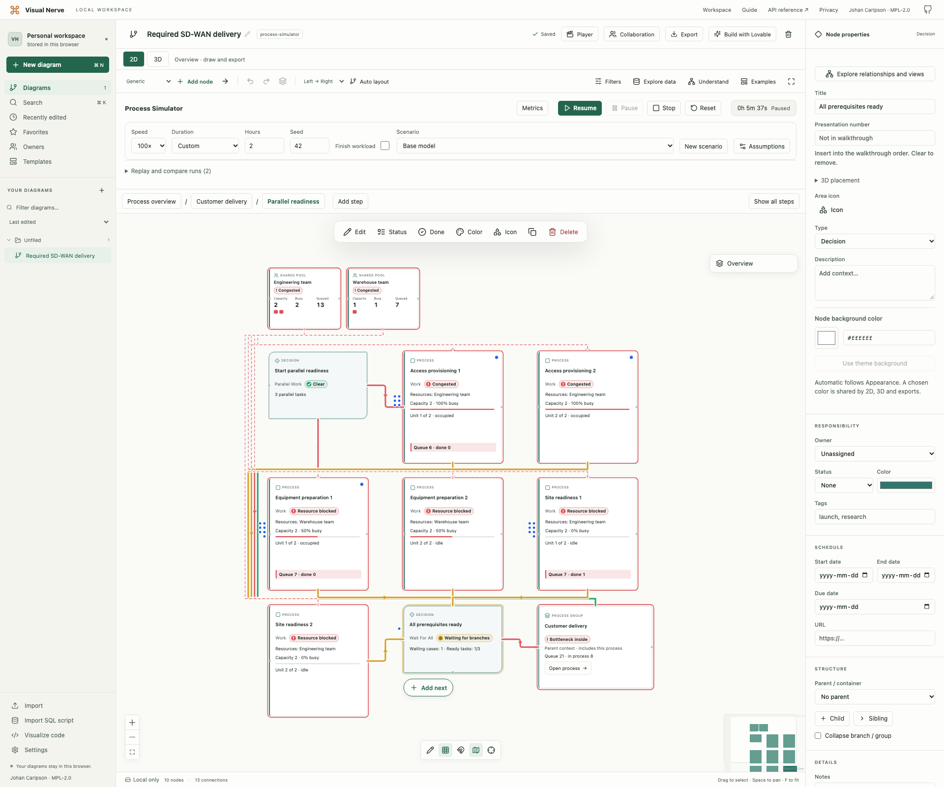
For a telecom delivery, access provisioning, equipment preparation and site readiness can happen at the same time. Installation must wait until all three are ready.
- Select an existing Source or Work step and use its + → Parallel work control. A complete block starts with two Work tasks and a Wait for all step. If the original step had a continuation, the block is inserted before it.
- Give each branch a useful name and configure its processing time, capacity, costs and shared resource requirements. Each branch has a real queue and can compete with other branches for the same staff.
- Use + → Work step on the Parallel work node to add another required branch. The new task is connected to the paired Wait for all node. Add intermediate steps with the normal connected-node control.
- Connect the Wait for all node to the next process step or Outcome. All outgoing connections from Parallel work are mandatory; every successful branch must reach its paired join.
- Play the model. The join shows the number of cases waiting and tasks ready. An early branch waits for the other tasks belonging to that same case, never for a different customer’s task.
The pictured example uses eight orders, three prerequisite tasks, shared engineers, a warehouse worker, installation and one billing outcome. Build the corresponding steps and shared resources in your own model, then review every rate, delay and cost in Assumptions. Add a scenario with two additional engineers to compare the reduction in waiting with the increased staffing cost.
Whole-system Created, Completed and In system count original cases. A case carries its revenue once; branch work still incurs its own processing and resource costs. Cycle time and time-to-revenue follow the original case’s simulation timestamps. If one branch fails or abandons, the case ends once, its other tasks are cancelled and their resources are released; already incurred costs remain.
A block supports 2–64 required branches and up to 16 nested parallel blocks. Paths inside a block must be acyclic and cannot cross into another block’s branches. Invalid pairs or connections show a validation error. A failure/rejection route may end the entire case; a successful Outcome belongs after the join. Assumptions → Nodes → Remove parallel block and all its tasks removes the selected fork/join and its enclosed tasks, reconnecting the incoming flow to the single continuation. Undo restores the complete edit. Review the button’s scope before removing a block.
The API and MCP guide shows the semantic pairing fields, live state and atomic model updates.
Outcomes: completion and realized revenue
Select an Outcome and choose completed, failed or rejected. Realize revenue determines whether it realizes the item’s carried expected revenue; Outcome revenue override can supply an explicit value.
Expected revenue is not cash already earned. Read the completed outcomes and realized revenue when evaluating results.
Scaling: extra capacity with delays and cost
Work and Resources have Automatic scaling → Enable scaling. Configure minimum/maximum capacity, scale increment, queue or utilization thresholds, low-utilization hold, startup/shutdown delays and cooldown.
Scaling is an assumption, not a visual duplication command. New capacity becomes available according to its delays. Scale-down respects active allocations, the configured minimum and the low-utilization period.
Scale up one-off cost adds a scaling charge. Extra unit cost / hour is a surcharge on extra units in addition to their regular hourly cost; it continues until those units scale down, including closed or idle periods.
A Resource’s minimum is the scaling floor when no separate scaling minimum is supplied. Invalid capacity combinations are rejected.
Improvements and investments
In improvements, choose Add improvement / investment, name it and select Activate improvement. Target a Work/Outcome node or a shared Resource.
Configure investment, operating cost, and supported processing/resource/capacity/cost/revenue modifiers. For example, a processing multiplier of 0.8 models processing at 80% of its previous duration, while a capacity increase adds actual slots or resource units within configured maxima.
Failure probability and Failure route represent an explicit failure assumption. A routed failure needs a valid outgoing connection from every affected Work node.
Resource improvements affect that resource: a staff resource reduction does not also reduce counters or Work slots. Processing/revenue/failure effects apply to Work nodes using that resource. Outcome improvements support economic and revenue effects, rather than nonexistent processing capacity.
Economics and the complete model
In economics, set the three-letter Currency, optional Maximum budget, and written Assumptions. A run exceeding its configured total budget fails with an explicit message.
Complete model exposes all semantic properties as JSON, including advanced configurations. Structured editors cover common assumptions. Validate the full draft before applying; malformed JSON does not become a partial saved model.
Control a run and compare like with like
| Control | Meaning |
|---|---|
| Play | Starts a run using the current captured assumptions and options. |
| Pause / Resume | Stops/resumes the current compatible run. |
| Rerun | Starts a new run when current assumptions/options differ. |
| Stop | Stops the current run. |
| Reset | Creates a new run and preserves the previous result. |
| Speed: 1× / 10× / 100× / MAX | Changes playback pacing; MAX processes events without waiting for animation. |
| Duration / Hours | Arrival/run horizon; presets include hour, day, week, 30-day month and 365-day year. |
| Seed | Reproducible random streams for stochastic arrivals and complexity. |
| Finish workload | Stops arrivals at the configured horizon and drains the existing work. |
A run freezes its model, scenario, seed and options. Later edits do not rewrite that result. If assumptions change during a run, the displayed metrics still belong to its original captured assumptions; Play starts a new run.
Changing the structure by adding or removing steps or connections, moving steps between subprocesses, or changing which shared resources they use detaches the old run from the canvas. An active run started with Play stops and keeps its actual partial result in Saved runs. Completed results stay unchanged; API/MCP runs continue independently against their captured model. Use Play to run the changed structure.
Changing speed does not improve business capacity or change the computed outcome. Use the same seed, horizon and finish-workload choice when comparing scenarios.
Create a scenario without rewriting the baseline
- Choose Base model in Scenario if you want to begin from the baseline.
- Choose New scenario and give it a meaningful name.
- Open Assumptions. Its context identifies the scenario you are editing.
- Change only the intended assumptions and choose Apply assumptions.
- Choose its duration/seed and run it.
- Compare with a captured baseline run.
New scenario can also start from the currently selected scenario. Scenarios keep explicit overrides instead of mutating Baseline. Scenario assumptions lets you change its Demand multiplier, rename or delete it. The multiplier scales all sources; change one Source in Assumptions when only one business flow should change.
For advanced JSON/API overrides, arrays replace their complete inherited value. JSON null removes an inherited optional property, such as a scaling rule; it cannot remove required fields, entity IDs or node types.
Interpret queues, capacity and metrics
In 2D, the canvas shows actual transit, queued work and busy/available capacity. Scaling can display Counter 1, Counter 2, Counter 3 as separate full cards. These are anonymous units of one logical object, not named employees or separately editable process nodes. The shared queue appears once. In the full flow (Show all steps for a diagram with subprocesses), you can move, resize and edit the original primary card. Additional capacity cards and the arranged overview/subprocess cards represent that same object; use Assumptions to change their shared processing rules or capacity.
Capacity visuals are limited to eight cards per bank and 256 extra cards across the view. More capacity is labeled as an aggregate and remains fully simulated. Particle snapshots are sampled; population metrics count all work.
3D keeps the logical model and live numeric metrics. Return to 2D for particles and full capacity banks. Runtime projections do not become extra saved model nodes.
The metrics dashboard explains the whole system:
| Metric | Meaning |
|---|---|
| Created / Completed / In system | Generated, completed and still-active population. |
| Abandoned / Failed | Work lost through waiting or failed processing/routing/constraints. |
| Current / Average / Maximum queue | Queue state and observed behavior over simulated time. |
| Throughput / hour | Observed completion rate. |
| Utilization / capacity / busy | Use of Work slots and shared resources. |
| Average / Median / P95 / P99 wait | Distribution of waiting time; tail values reveal cases an average can hide. |
| TTR | Time from creation to revenue realization. |
| Cycle time | Time through the modeled process. |
| Expected / Revenue / Lost revenue | Potential value, realized value and separately reported lost value. |
| Cost | Operating, resource and scaling cost. |
| Contribution | Realized revenue minus those costs. |
| Investment / Cash impact | Investment and the cumulative result after investment. |
Open Bottlenecks, shared resources and particle types for resource/type detail. Bottlenecks rank observed queues, waiting and utilization; they can migrate after a change.
A P95 wait of five minutes means about 95% of observed waits are five minutes or less; P99 describes the 99th percentile. They expose the slower tail. P95 requires at least 20 observations and P99 at least 100; otherwise the value is unavailable. Large populations use bounded approximate distributions with disclosed precision. Type-level costs can exclude idle capacity, fixed investments or system overhead, so summing type costs need not equal whole-system cost.
Replay and compare saved results
- Open Replay & compare on a compact screen, or the desktop run comparison section.
- Choose a Saved run.
- Pause a running run before using Replay time.
- Set a simulated time and choose Inspect this moment.
- Select two or more saved runs and choose Compare selected runs.
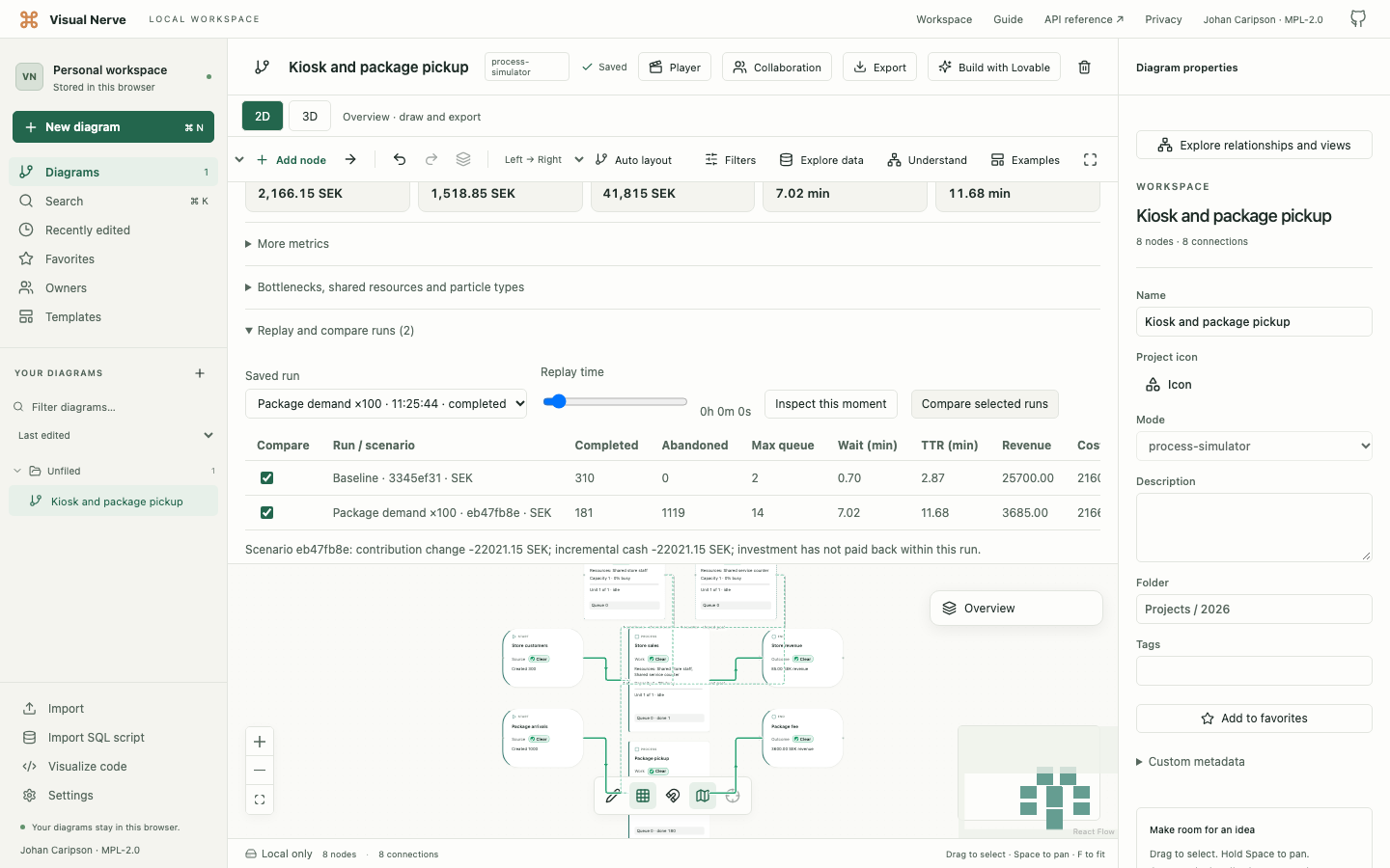
Comparison shows deltas, incremental cash and observed payback. “Investment has not paid back within this run” means the simulated cash did not cross the investment during that horizon; it does not invent a future payback date.
Saved runs keep their captured scenario name and currency, even if you later rename or delete the scenario or change the document currency. Compare runs with the same captured currency. Comparisons reject different currencies and do not convert exchange rates.
Replay reconstructs captured inputs deterministically rather than relying on every animation frame being retained. Saved results remain associated with their original assumptions.
A simple check of your understanding
To reason about a minimal model, configure ten initially arriving items, one Work slot, one-minute processing, zero travel, no abandonment and a completed revenue outcome of 100 per item. Use Finish workload.
Expected result: ten completions, 1,000 realized revenue and the last completion after ten simulated minutes. Then use two Work slots and compare the captured results. If you add one shared employee required by both slots, that resource becomes the constraint again.
This exercise tests the assumptions you entered; it does not require AI or the local bridge.
Persistence, headless runs and safety limits
Models, scenarios and bounded run archives stay in local IndexedDB. Native JSON, history/duplication and complete backup preserve their supported simulator content. Runtime card projections remain temporary. Keep a backup before changing browser or device.
MAX/headless can run without a selected diagram or animation. The connected browser must remain open for local storage and worker execution. Closing it ends execution; reopening preserves saved models/results, and captured runs support deterministic replay.
The optional API/MCP integration
uses the same model and engine for assumptions, scenarios, runs, controls, replay, metrics, queues, events and comparison. Start with visual_nerve_api_docs and GET /simulation/capabilities. Inspection/comparison permit read-only access; changes and external execution/replay require write access. Revoking the grant stops externally initiated execution without rewriting saved results.
Limits describe bounded execution, not guaranteed interactive speed:
- Up to 50,000 semantic nodes and 200,000 flow edges; maximum configured horizon ten simulated years.
- Up to 200,000 simultaneously active particles, 50 million scheduled/semantic events per run and 10,000 route visits per particle.
- Long route labels are summarized with a stable identifier and connection count. Parallel task histories do not need to retain every repeated connection; full-population counts, costs and time-to-revenue remain unchanged.
- Four resident execution/replay workers, including paused workers and startup reservations; sixty cached runs.
- Up to 30 archived runs per diagram. Default retained samples/events are 300/2,000, configurable to at most 10,000/100,000.
- Up to 240 checkpoints per run. Replay can reconstruct captured inputs without retaining every frame.
Exceeding an execution limit fails explicitly with partial metrics; it does not silently discard work and report success. Event pages disclose retained/dropped counts while population metrics remain complete.
Common questions
| Question | Check |
|---|---|
| Why did hiring more people not increase throughput? | Inspect other required resources, Work slots, schedules, routing and the current bottleneck. |
| Why are items abandoning? | Compare queue length, patience, available capacity and overflow route. |
| Why did metrics not change after editing? | They still describe the captured run. Play/Rerun creates a run with the new assumptions. |
| Why do week runs stop generating after one day? | Check repeating schedules and an unintended Maximum arrivals cap. |
| Why is cost higher than busy time suggests? | Available capacity costs include idle time; extra scaling units can carry continuous surcharges. |
| Why are there fewer animated items than Created? | Visual samples are bounded; metrics cover the whole population. |
| Why did the run stop with an error? | Read the message for budget, topology or execution limits before starting a revised run. |
| Why can I not apply settings? | Fix invalid JSON/semantic references, or reopen a draft made stale by another change. |
Continue with Editing diagrams for native cards and connections, Presentations to explain the model, or Sharing and export to preserve and communicate it.