Open the workspace and choose New diagram → Process Simulator. Follow the complete simulator guide .
Start with the whole-system question
A kiosk serves 300 store customers and 10 package customers per opening day. Store purchases take two minutes; package pickup takes four. Both require the same employee and counter.
At low package volume, the flows can coexist. Change package demand to 1,000 per day and that extra work competes with the store’s existing business. Waiting, abandonment and lost store revenue can increase even when each completed package earns a fee.
The bundled example uses an explicit 12-hour opening day, repeating schedules, evenly spaced arrivals, patience thresholds, travel time and paid staff. You can inspect and change every assumption.
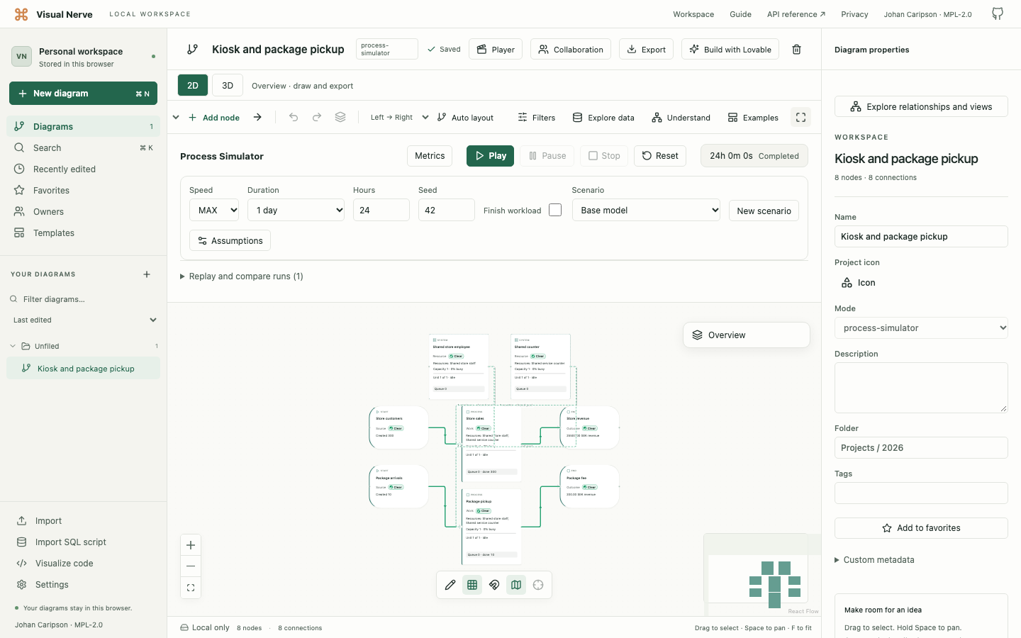
Model work, processing and shared capacity
| Model element | What it means |
|---|---|
| Particle type | A customer, order, package or other work item with revenue, complexity, priority and patience. |
| Source | Arrivals, bursts, schedules and maximum counts. |
| Work | Processing time, parallel slots, queue behavior and required resources. |
| Router | A permitted choice based on configured rules, attributes or actual state. |
| Resource | Shared employees, counters, machines, storage or other constrained capacity. |
| Outcome | Completed, failed or rejected work, with optional realized revenue. |
Multiple Work nodes can require the same logical resource. Adding another processing card does not automatically add another employee. Resource contention is part of the calculation.
Open the process to find the constrained step
Build a main process with nested subprocesses through guided setup, or group an existing model under Assumptions → Processes. Each real Work step has its own time, capacity, cost and resource requirements. Group cards summarize actual queues, work in progress, cycle time and the named constraint; opening a group reveals its children.
The Delivery network + returns example connects order acceptance, planning, warehouse preparation, transport, installation, billing and returns. Its flows share operations staff, technicians, engineers, drivers and a loading dock. Compare a returns rush or additional warehouse and delivery capacity to see how pressure travels across the business.
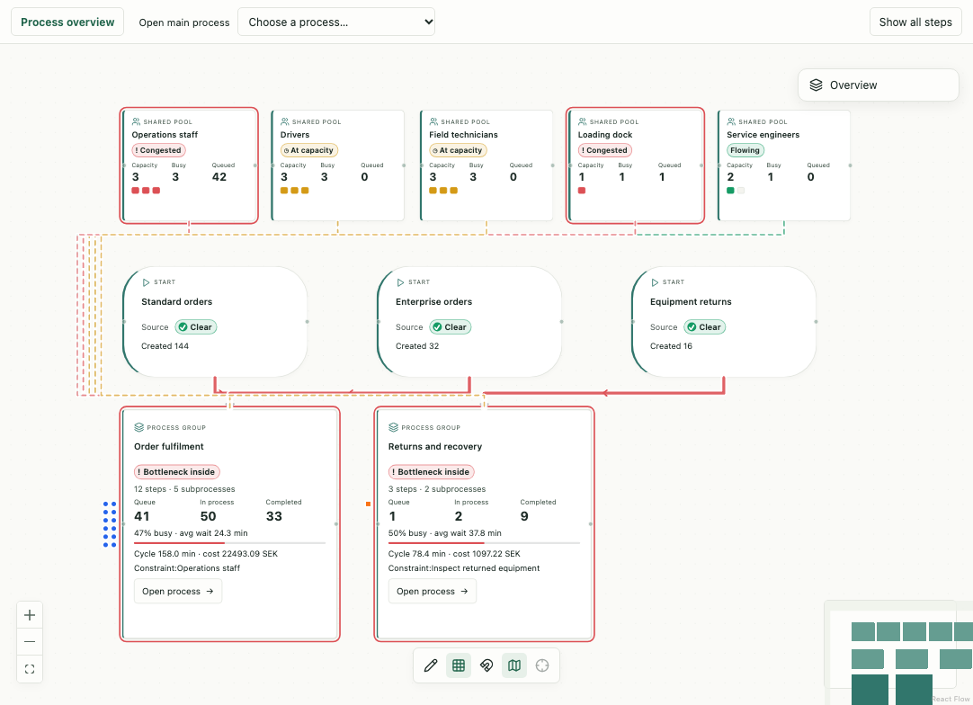
Groups add no processing or charge. A parent’s values include its subprocesses, so parent and child totals overlap. Full-system results remain the reference for economic comparisons. Show all steps, 3D and export retain the complete underlying flow.
Choose an infrastructure capacity example
The same engine also supports four editable starting points:
| Template | Explicit assumptions |
|---|---|
| API & Compute Capacity | Dedicated CPU cores and core-seconds, retained/stage RAM and an atomic database connection pool |
| Network & Multi-Site Capacity | Payload bytes, shared Mbps and separately entered propagation delay across sites |
| Energy & Power Capacity | Generation windows, bounded grid import, battery rates/efficiencies and actual delivered energy |
| Datacenter Capacity | WAN, retained RAM, concurrent CPU and explicit energy-budget branches, joined before database work |
Opening a template goes through normal browser storage acceptance and, on the isolated app, local unlock. It creates an editable local diagram; visiting this public page creates no workspace data. The examples use synthetic inputs rather than measured server/network/power performance. Follow the infrastructure guide before changing quantities or comparing scenarios.
Model 2 Work and all resource pools show one aggregate logical card. Work capacity limits in-flight jobs rather than physical server replicas. Legacy model 1 capacity-card banks retain their existing meaning. The models describe allocation, fluid payload sharing and energy balance; they do not implement an operating-system scheduler, TCP or AC electrical solver.
Observe the constraint on the canvas
In 2D, particles follow valid model connections and remain queued until processing can begin. Node indicators and metrics reveal busy capacity, waiting and saturation. A bottleneck is identified from observed state and can move when you remove an earlier constraint.
In legacy model 1, configured scaling can show additional capacity cards, such as Counter 1, Counter 2 and Counter 3. They represent units of one logical node or resource, with a shared queue. They are temporary capacity visuals, not separately saved employee identities. Infrastructure model 2 keeps aggregate logical cards instead.
Rendering is bounded: large populations use samples or aggregation while metrics describe all simulated work. The full live particle and capacity-bank view is in 2D; 3D retains the logical diagram and numeric metrics.
Change an assumption and compare another run
- Run the baseline with a chosen duration and seed.
- Create a scenario without replacing the baseline.
- Open Assumptions and change a source rate, processing time, resource or capacity rule.
- Apply the draft and run it.
- Compare saved results using the same horizon, seed and finish-workload choice.
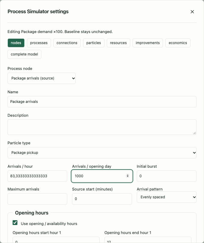
The kiosk includes scenarios for higher package demand, a dedicated package employee, and additional package employees with a dedicated counter. Each intervention applies its configured cost; it does not simply make throughput better for free.
Read economics alongside throughput
Inspect created, completed and abandoned work; queue length and waiting percentiles; resource utilization; throughput; realized and lost revenue; operating, resource and scaling cost; contribution; and time-to-revenue.
Improvements can add an investment and change processing or capacity. Comparison reports incremental cash impact and observed payback when the simulated result crosses the investment. A run that has not paid back within its horizon is reported as such.
These are consequences of the assumptions you supplied. The simulator does not validate those assumptions against a real business or promise a financial outcome.
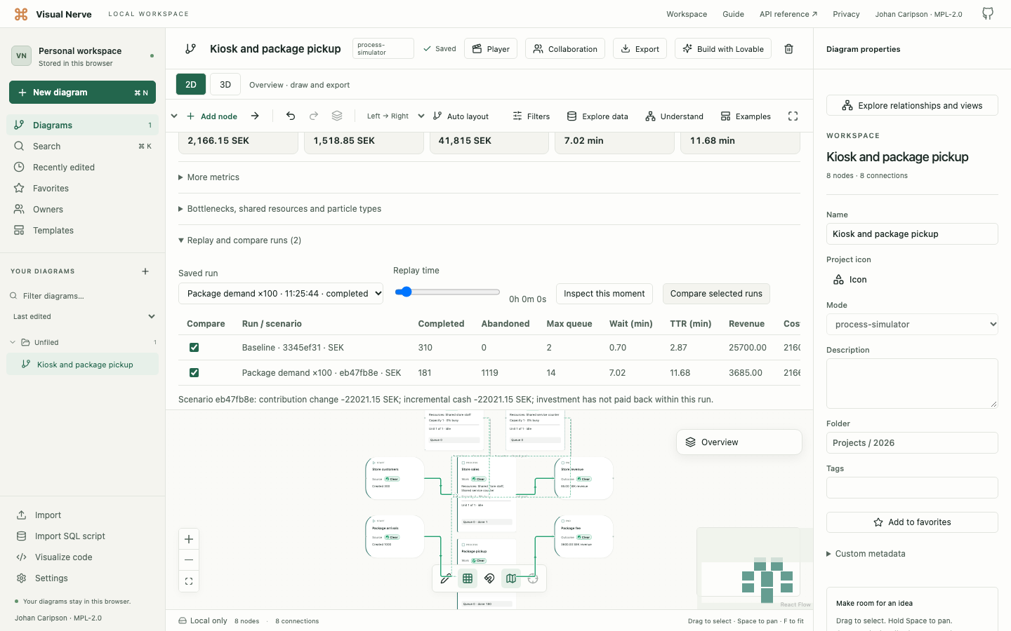
Replay and automate the same model
Play, pause, stop, reset and choose 1×, 10×, 100× or MAX. Simulation time is independent of browser wall-clock time. MAX processes events without waiting for particle animation.
The discrete-event engine uses seeded randomization. The same captured model, scenario, seed and options produce the same business metrics through UI, REST or MCP. Runs retain their captured inputs, so later edits do not rewrite previous results. Replay lets you inspect an earlier simulated moment.
API and MCP expose semantic models, queues, resources, events, metrics, scenarios and controls. A client can run sequential demand multipliers and compare separately identified results. Headless execution needs no active canvas, but the browser must remain open and connected for local workers and storage.
Keep the model and its limits visible
Models, scenarios and bounded run archives are stored in local IndexedDB. Back up work before changing browser, device or website origin. No mandatory backend or cloud database is required.
Execution has explicit limits for topology, active particles, events, route visits, workers and retained results. Exceeding a limit produces an error with partial metrics, rather than silently dropping work and reporting success. Discover the current ceilings through the API or the guide.
Create a Process Simulator · Modeling and troubleshooting guide · Programmatic control